Preface
This tutorial was made solely for the purpose of education and it was designed for students taking Applied Math 0330. It is primarily for students who have very little experience or have never used Mathematica and programming before and would like to learn more of the basics for this computer algebra system. As a friendly reminder, don't forget to clear variables in use and/or the kernel. The Mathematica commands in this tutorial are all written in bold black font, while Mathematica output is in normal font.
Finally, you can copy and paste all commands into your Mathematica notebook, change the parameters, and run them because the tutorial is under the terms of the GNU General Public License (GPL). You, as the user, are free to use the scripts for your needs to learn the Mathematica program, and have the right to distribute this tutorial and refer to this tutorial as long as this tutorial is accredited appropriately. The tutorial accompanies the textbook Applied Differential Equations. The Primary Course by Vladimir Dobrushkin, CRC Press, 2015; http://www.crcpress.com/product/isbn/9781439851043
Return to computing page for the second course APMA0340
Return to Mathematica tutorial for the second course APMA0340
Return to Mathematica tutorial for the first course APMA0330
Return to the main page for the second course APMA0340
Return to the main page for the first course APMA0330
Return to Part III of the course APMA0330
Glossary
Hamming Method
In 1959, Richard Wesley Hamming (1915--1998) from Bell Telephone Laboratories, Murray Hill, New Jersey, proposed a stable predictor-corrector method for ordinary differential equations, which now bears his name. He improved classical Milne--Simpson method by replacing unstable corrector rule by a stable one.
Journal of the ACM, Volume 6, Issue 1, Jan. 1959, pages 37--47.
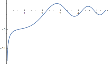
Example. Let us start with the Riccati equation \( y' = x^2 + y^2 \) subject to the initial condition \( y(0) =-1 . \) Its solution is expressed through Bessel functions:
Plot[d[x], {x, 0, 5.5}, PlotStyle -> Thick]
Program (Hamming method): to approximate the solution of the initial value problem \( y' = f(x,y) , \ y(a) = y_0 \) over the interval [a,b] by using the predictor
function H=hamming(f,T,Y)
% Input  -- f is the slope function entered as a string 'f'
%        -- T is the vector of abscissas
%        -- Y is the vector of ordinates
% Remark -- the first four coordinates of T aand Y must have starting values obtained with RK4

% Output -- H=[T',Y'] where T is the vector of abscissas; Y is the vector of ordinates
n=length(T);
if n<5, break,end;
F=zeros(1,4);
F=feval(f,T(1:4),Y(1:4));
h=T(2)-T(1);
pold=0;
cold=0;
for k=4:n-1
    % predictor
    pnew=Y(k-3)+(4*h/3)*(F(2:4)*[2 -1 2]');
    % modifier
    pmod=pnew+112*(cold-pold)/121;
    T(k+1)=T(1)+h*k;
    F=[F(2) F(3) F(4) feval(f,T(k+1),pmod)];
    % corrector
    cnew=(9*Y(k)-Y(k-2)+3*h*(F(2:4)*[-1 2 1]'))/8;
    Y(k+1)=cnew+9*(pnew-cnew)/121;\
    pold=pnew;
    cold=cnew;
    F(4)=feval(f,T(k+1),Y(k+1));
end
H=[T' Y'];
Return to Mathematica page
Return to the main page (APMA0330)
Return to the Part 1 (Plotting)
Return to the Part 2 (First Order ODEs)
Return to the Part 3 (Numerical Methods)
Return to the Part 4 (Second and Higher Order ODEs)
Return to the Part 5 (Series and Recurrences)
Return to the Part 6 (Laplace Transform)
Return to the Part 7 (Boundary Value Problems)