Preface
This section is devoted to the Euler method and some of its modifications. In 1768, Leonhard Euler (pronounced "oiler" not "youler") published (St. Petersburg, Russia) an article where he introduced the tangent line method, now bearing his name. This method not only gave birth to numerical discrete methods such as Runge--Kutta, but also promoted theoretical research, including Cauchy--Lipschitz method.
Return to computing page for the second course APMA0340
Return to Mathematica tutorial for the second course APMA0340
Return to the main page for the course APMA0330
Return to the main page for the course APMA0340
Return to Part III of the course APMA0330
Glossary
Euler's Methods

We start with the first numerical method for solving initial value problems that bears Euler's name (correct pronunciation: oiler not uler). Leonhard Euler was born 1707, in Basel, Switzerland and passed away 1783, in Saint Petersburg, Russia. In 1738, he became almost blind in his right eye. Euler was one of the most eminent mathematicians of the 18th century, and is held to be one of the greatest in history. He is also widely considered to be the most prolific mathematician of all time. He spent most of his adult life in Saint Petersburg, Russia, except about 20 years in Berlin, then the capital of Prussia.
In 1768, Leonhard Euler (St. Petersburg, Russia) introduced a numerical method that is now called the Euler method or the tangent line method for solving numerically the initial value problem:
To start, we need mesh or grid points, that is, the set of discrete points for an independent variable at which we find approximate solutions. In other words, we will find approximate values of the unknown solution at these mesh points. For simplicity, we use uniform grid with fixed step length h; however, in practical applications, it is almost always not a constant. For convenience, we subdivide the interval of interest [𝑎,b] (where usually 𝑎 = x0 is the starting point) into m equal subintervals and select the mesh/grid points
There are three main approaches (we do not discuss others in this section) to derive the Euler rule: either use finite difference approximation to the derivative or transfer the initial value problem to the Volterra integral equation and then truncate it, or apply Taylor series.
- We start with the finite difference method. It is known that numerical differentiation is an ill-posed problem that does not depend continuously on the data. If we approximate the derivative in the left-hand side of the differential equation y' = f(x,y) by the
finite difference
\[ y' (x_n ) \approx \frac{y_{n+1} - y_n}{h} \]on the small subinterval \( [x_{n+1} , x_n ] , \) we arrive at the Euler's rule when the slope function is evaluated at x = xn.\begin{equation*} y_{n+1} = y_n + (x_{n+1} - x_n ) f( x_n , y_n ) \qquad \mbox{or} \qquad y_{n+1} = y_n + h f_n , \end{equation*}where the following notations are used: \( h=x_{n+1} - x_n \) is the step length (which is assumed to be constant for simplicity), \( f_n = f( x_n , y_n ) \) is the value of slope function at mesh point, and yn denotes the approximate value of the actual solution y = ϕ(x) at the point \( x_n = x_0 + n\,h \) (\( n=1,2,\ldots \) ).
- Integrating the identity y'(x) = f(x,y(x)) between xn and xn+1, we obtain
Such integration transfers the initial value problem for unbounded derivative operator into the integral equation, avoiding a discontinuous operator. Approximating the integral by the left rectangular (very crude) rule for numerical integration (length of interval times value of integrand at left end point) and identifying \( y(x_n ) \) with yn, we again obtain the Euler formula.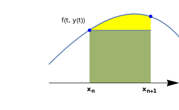 curve = Plot[x - Exp[x - 0.05] + 1.5, {x, -1.0, 0.7}, PlotStyle -> Thick, Axes -> False, Epilog -> {Blue, PointSize@Large, Point[{{-0.5, 0.42}, {0.25, 0.53}}]}, PlotRange -> {{-1.6, 0.6}, {-0.22, 0.66}}];
line = ListLinePlot[{{-0.5, 0.42}, {0.25, 0.42}}, Filling -> Bottom, FillingStyle -> Opacity[0.6]];
curve2 = Plot[x - Exp[x - 0.05] + 1.5, {x, -0.5, 0.25}, PlotStyle -> Thick, Axes -> False, PlotRange -> {{-1.6, 0.6}, {0.0, 0.66}}, Filling -> Bottom, FillingStyle -> Yellow];
ar1 = Graphics[{Black, Arrowheads[0.07], Arrow[{{-1.0, 0.0}, {0.6, 0.0}}]}];
t1 = Graphics[ Text[Style["f(t, y(t))", FontSize -> 12], {-0.7, 0.5}]]; xn = Graphics[ Text[Style[Subscript["x", "n"], FontSize -> 12, FontColor -> Black, Bold], {-0.48, -0.05}]];
xn1 = Graphics[ Text[Style[Subscript["x", "n+1"], FontSize -> 12, FontColor -> Black, Bold], {0.24, -0.05}]];
Show[curve, curve2, line, ar1, t1, xn, xn1]\[ y(x_{n+1}) - y(x_n ) = \int_{x_n}^{x_{n+1}} f(t, y(t))\,{\text d} t . \] - We may assume the possibility of expanding the solution in a Taylor series around the point xn:
\[ y(x_{n+1}) = y(x_n +h) = y(x_{n}) + h\, f(x_n, y(x_n )) + \frac{1}{2}\, h^2 \,y'' (x_n ) + \cdots . \]The Euler formula is the result of truncating this series after the linear term in h: yn+1 = yn + h f(xn, yn).
 |
curve = Plot[x - Exp[x - 0.05] + 1.5, {x, -1.0, 0.7},
PlotStyle -> Thick, Axes -> False,
Epilog -> {Blue, PointSize@Large, Point[{{-0.4, 0.46}, {-0.4, 0.5}, {0, 0.63}, {0, 0.55}, {0.4, 0.48}, {0.4, 0.61}}]}, PlotRange -> {{-1.6, 0.6}, {-0.22, 0.66}}] line1 = Graphics[Line[{{-0.8, 0.27}, {-0.4, 0.5}}]]; line2 = Graphics[{Dashed, Line[{{-0.8, 0.27}, {-0.8, -0.16}}]}]; line2a = Graphics[{Dashed, Line[{{-0.8, 0.27}, {-1.5, 0.27}}]}]; line3 = Graphics[{Dashed, Line[{{-0.4, 0.46}, {-0.4, -0.16}}]}]; line3a = Graphics[{Dashed, Line[{{-0.4, 0.46}, {-1.5, 0.46}}]}]; line4 = Graphics[{Dashed, Line[{{0.0, 0.55}, {0.0, -0.16}}]}]; line4a = Graphics[{Dashed, Line[{{0.0, 0.55}, {-1.5, 0.55}}]}]; line5 = Graphics[{Dashed, Line[{{0.4, 0.48}, {0.4, -0.16}}]}]; ar1 = Graphics[{Black, Arrowheads[0.07], Arrow[{{-1.5, -0.22}, {-1.5, 0.65}}]}]; ar2 = Graphics[{Black, Arrowheads[0.07], Arrow[{{-1.5, -0.16}, {0.6, -0.16}}]}]; aa1 = Graphics[{Arrowheads[{-0.04, 0.04}], Arrow[{{-0.8, 0}, {-0.4, 0}}]}]; aa2 = Graphics[{Arrowheads[{-0.04, 0.04}], Arrow[{{-0.4, 0}, {-0.0, 0}}]}]; aa3 = Graphics[{Arrowheads[{-0.04, 0.04}], Arrow[{{0.0, 0}, {0.4, 0}}]}]; t1 = Graphics[Text[Style["h", FontSize -> 12], {-0.6, 0.05}]]; t2 = Graphics[Text[Style["h", FontSize -> 12], {-0.6, 0.05}]]; t3 = Graphics[Text[Style["h", FontSize -> 12], {0.2, 0.05}]]; x0 = Graphics[ Text[Style[Subscript["x", "0"], FontSize -> 12, FontColor -> Black, Bold], {-0.78, -0.19}]]; x1 = Graphics[ Text[Style[Subscript["x", "1"], FontSize -> 12, FontColor -> Black, Bold], {-0.38, -0.19}]]; x2 = Graphics[ Text[Style[Subscript["x", "2"], FontSize -> 12, FontColor -> Black, Bold], {0.02, -0.19}]]; x3 = Graphics[ Text[Style[Subscript["x", "3"], FontSize -> 12, FontColor -> Black, Bold], {0.42, -0.19}]]; x = Graphics[ Text[Style["x", FontSize -> 12, FontColor -> Black, Bold], {0.5, -0.09}]]; y = Graphics[ Text[Style["y", FontSize -> 12, FontColor -> Black, Bold], {-1.4, 0.6}]]; line6 = Graphics[Line[{{-0.4, 0.5}, {0.0, 0.63}}]]; y0 = Graphics[ Text[Style[Subscript["y", "0"], FontSize -> 12, FontColor -> Black, Bold], {-0.7, 0.26}]]; y1 = Graphics[ Text[Style[Subscript["y", "1"], FontSize -> 12, FontColor -> Black, Bold], {-0.47, 0.5}]]; y2 = Graphics[ Text[Style[Subscript["y", "2"], FontSize -> 12, FontColor -> Black, Bold], {0.09, 0.63}]]; y3 = Graphics[ Text[Style[Subscript["y", "3"], FontSize -> 12, FontColor -> Black, Bold], {0.35, 0.58}]]; tr = Graphics[ Text[Style["true value", FontSize -> 12, FontColor -> Black, Bold], {-1.2, 0.42}]];; Show[curve, line1, line2, line3, line2a, line3a, line4, line4a , \ line5, ar1, ar2, aa1, aa2, aa3, t1, t2, t3, x0, x1, x2, x3, x, y, \ line6, y0, y1, y2, y3,tr] |
|
\[
y_{n+1} = y_n + h\, f(x_{n}, y_{n}) , \qquad y_0 = y(0), \qquad n=0,1,2,\ldots .
\]
|
|---|
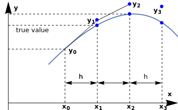
Therefore, every next Euler point yn+1 is determined according to the tangent line starting from the previous grid point (xn,yn) with slope f(xn,yn); recall that the equation of the tangent line is y = yn + f(xn,yn) (x - xn). If we connect all grid points generated by the Euler algorithm
 |
euler = Plot[{x/3, -x/3}, {x, -1, 1}, Axes -> False,
AspectRatio -> 1/3, PlotStyle -> {{Thick, Red}, {Thick, Red}}];
line = Graphics[{Thick, Line[{{-1, 0.2}, {-0.8, 0.2}, {-0.6, 0}, {-0.4, -0.1}, {-0.2, -0.0 .5}, {0, 0}, {0.2, 0.01}, {0.4, 0.1}, {0.6, 0.15}, {0.8, 0.1}, {1.0, 0.2}}]; point = Graphics[{PointSize[Large], Point[{{-1, 0.2}, {-0.8, 0.2}, {-0.6, 0}, {-0.4, -0.1}, {-0.2, -0.0 .5}, {0, 0}, {0.2, 0.01}, {0.4, 0.1}, {0.6, 0.15}, {0.8, 0.1}, {1.0, 0.2}}]}]; Show[line, euler, point] |
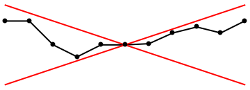
Suppose that \( |f| \le M, \) where M is a positive constant. In this case the segments in the Euler polygon have slopes between -M and M and the polygon lies between two lines of slopes ±M through the point (x0, y0). It is natural to assume that the solution has the same property. This surmise can be proved without using the Euler polygon and without assuming that the solution is unique (Cauchy--Lipschitz theorem).
This algorithm can be accomplished either directly
y[0] = 1/2; h = 0.1; f[x_, y_] = y^2 - x^2;
Do[y[n + 1] = y[n] + h f[h n, y[n]], {n, 0, 10}]
y[5] (* to obtain the fifth numerical value *)
Block[{ xold=x0,
yold=y0,
sollist={{x0,y0}},h},
h=N[(xn-x0)/steps];
Do[ xnew=xold+h;
ynew=yold+h*(f/.{x->xold,y->yold});
sollist=Append[sollist,{xnew,ynew}];
xold=xnew;
yold=ynew,
{steps}
];
Return[sollist] (* to see all grid points *)
]
x = x /. First[
NDSolve[{x'[t] == x[t]*x[t] - t^2, x[0] == 1/2}, x, {t, 0, 1}, StartingStepSize -> 0.11,
Method -> {"FixedStep", Method -> "ExplicitEuler"}]];
grid = Table[{t, x[t]}, {t, 0, 1, 0.1}]
ListLinePlot[grid]
Example: We illustrate how the Euler method works on an example of a linear equation when all calculations become transparent. Note that Mathematica attempts to solve the ODE using its function. A solution may or may not be possible using this function. In the case when a solution may not be known or determined, Euler's method provides an alternative to approximate the solution numerically. Consider the initial value problem:
Let us check a few first terms:
DiscretePlot[sol, {n, 0, 27}, PlotStyle -> {PointSize[0.02]}]
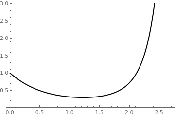
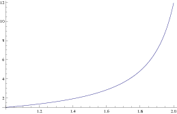
soldif = NDSolve[{y'[x] == x^2 *y[x] - 1.5*y[x], y[0] == 1}, y, {x, 0, 2.8}]
Plot[Evaluate[y[x]] /. soldif, {x, 0, 2.7}, PlotStyle -> {Black, Thick}, PlotRange -> {0, 3}]
 |
 |
| Euler's discrete approximation | True solution |
x0 := 0 (* starting point in x *)
y0 := 0 (* starting value for y *)
xf=2.0; (* Value of x at which y is desired *)
h = (xf - x0)/5.0 (* step size in x *)
plot = Plot[Evaluate[y[x] /. soln], {x, x0, xf},
PlotStyle -> {{Thickness[0.01], RGBColor[1, 0, 0]}}]
X[1] = X[0] + h
Y[1] = Y[0] + f[X[0], Y[0]]*h
plot1 = ListPlot[{{X[0], Y[0]}, {X[1], Y[1]}}, Joined -> True,
PlotStyle -> {Thickness[0.005], RGBColor[0, 0, 1]}, DisplayFunction -> Identity]
Y[2] = Y[1] + f[X[1], Y[1]]*h
plot2 = ListPlot[{{X[0], Y[0]}, {X[1], Y[1]}, {X[2], Y[2]}}, Joined -> True,
PlotStyle -> {Thickness[0.005], RGBColor[0, 0, 1]}, DisplayFunction -> Identity]
Y[3] = Y[2] + f[X[2], Y[2]]*h
plot3 = ListPlot[{{X[0], Y[0]}, {X[1], Y[1]}, {X[2], Y[2]}, {X[3], Y[3]}}, Joined -> True,
PlotStyle -> {Thickness[0.005], RGBColor[0, 0, 1]}, DisplayFunction -> Identity]
Y[4] = Y[3] + f[X[3], Y[3]]*h
plot4 = ListPlot[{{X[0], Y[0]}, {X[1], Y[1]}, {X[2], Y[2]}, {X[3], Y[3]}, {X[4], Y[4]}}, Joined -> True,
PlotStyle -> {Thickness[0.005], RGBColor[0, 0, 1]}, DisplayFunction -> Identity]
In the above codes, a special option DisplayFunction was used. You can either remove this option or replace with a standard one: DisplayFunction -> $DisplayFunction. All Mathematica graphics functions such as Show and Plot have an option DisplayFunction,which specifies how the Mathematica graphics and sound objects they produce should actually be displayed. The way this works is that the setting you give for DisplayFunction is automatically applied to each graphics object that is produced.
DisplayFunction -> Identity generate no display
DisplayFunction -> f apply f to graphics objects to produce display
Within the Mathematica kernel, graphics are always represented by graphics objects involving graphics primitives. When you actually render graphics, however, they must be converted to a lower-level form which can be processed by a Mathematica front end, such as a notebook interface, or by other external programs. The standard low-level form that Mathematica uses for graphics is PostScript. The Mathematica function Display takes any Mathematica graphics object, and converts it into a block of PostScript code. It can then send this code to a file, an external program, or in general any output stream.
| n | xn | yn | Exact solution | Absolute error |
|---|---|---|---|---|
| 1 | 0.1 | 0.85 | 0.860995 | 0.0109949 |
| 2 | 0.2 | 0.72335 | 0.742796 | 0.0194464 |
| 3 | 0.3 | 0.617741 | 0.643393 | 0.0256518 |
| 4 | 0.4 | 0.530639 | 0.560645 | 0.030006 |
| 5 | 0.5 | 0.459534 | 0.492464 | 0.0329305 |
| 6 | 0.6 | 0.402092 | 0.436922 | 0.0348302 |
| 7 | 0.7 | 0.356254 | 0.392324 | 0.0360707 |
| 8 | 0.8 | 0.320272 | 0.357245 | 0.0369731 |
| 9 | 0.9 | 0.292729 | 0.330549 | 0.0378206 |
| 10 | 1.0 | 0.27253 | 0.311403 | 0.0388729 |
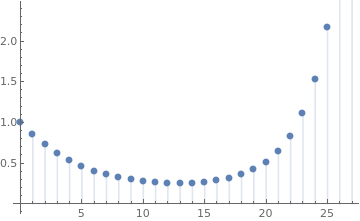
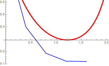
Example: Consider the initial value problem for the logistic equation
y[1] = y[0] + h*y[0]*(1 - y[0])
Do[y[n] = y[n - 2] + 2*h*y[n - 1]*(1 - y[n - 1]), {n, 2, 500}]
ListPlot[Table[{n*h, y[n]}, {n, 0, 500}]]
Another approach is based on transferring the given IVP \( y' = f(x,y) , \quad y(x_0 ) = y_0 \) to an equivalent integral equation
y[0] = 0.5; h = 0.1; f[y_] = y^2 - y;
Do[y[n + 1] = y[n] + h f[y[n]], {n, 0, 500}]
y[1]
| n | xn | yn | Exact solution | Absolute error |
|---|---|---|---|---|
| 1 | 0.1 | 0.475 | 0.524979 | 0.0499792 |
| 2 | 0.2 | 0.450063 | 0.549834 | 0.0997715 |
| 5 | 0.5 | 0.376852 | 0.622459 | 0.245607 |
| 10 | 1.0 | 0.266597 | 0.731059 | 0.464462 |
| 20 | 2.0 | 0.114573 | 0.880797 | 0.766224 |
| 30 | 3.0 | 0.0435246 | 0.952574 | 0.90905 |
| 50 | 5.0 | 0.00552563 | 0.993307 | 0.987782 |
| 100 | 10.0 | 0.0000286528 | 0.999955 | 0.999926 |
| 200 | 20.0 | 7.61083×10⁻¹⁰ | 1. | 1. |
| 400 | 40.0 | 5.3695×10⁻¹⁹ | 1. | 1. |
Example: We consider the following initial value problem for the Riccati equation
DSolve:
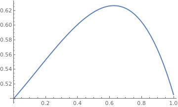 |
explicit = DSolve[{y'[x] == y[x]^2 - x^2 , y[0] == 1/2}, y, x]
Since the expression for the explicit solution involves special functions, we just evaluate its one particular value at x = 0.5 and plot the function
true[x_] = y[x] /. explicit
true[0.5]
{0.617769 + 2.77556*10^-17 I}
Plot[true[x], {x, 0, 1}, PlotStyle -> Thick]
|
euler:
| n | xn | yn | Exact solution | Absolute error |
|---|---|---|---|---|
| 1 | 0.1 | 0.525 | 0.525974 | 0.000973594 |
| 2 | 0.2 | 0.551563 | 0.552738 | 0.0011751 |
| 3 | 0.3 | 0.577985 | 0.578417 | 0.000432741 |
| 4 | 0.4 | 0.602391 | 0.600901 | -0.00149051 |
| 5 | 0.5 | 0.62267 | 0.617769 | -0.00490958 |
| 6 | 0.6 | 0.636452 | 0.626228 | -0.0102239 |
| 7 | 0.7 | 0.640959 | 0.623052 | -0.0179072 |
| 8 | 0.8 | 0.633042 | 0.604575 | -0.028467 |
| 9 | 0.9 | 0.609116 | 0.566763 | -0.0423522 |
| 10 | 1.0 | 0.565218 | 0.505431 | -0.0597873 |
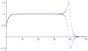
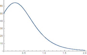
Example: To demonstrate the latter approach, we consider the initial value problem for the integro-differential equation
For the general step in Euler's rule, we have
T[0] := h^2 *50^2
y[0] := 50
y[1] := y[0] + 2.3*h*50 - 0.01*h*50^2 - 0.1*h^2*50^2
Do[ T[k] = T[k - 1] + h*(y[k] + y[k - 1])/2;
y[k + 1] = y[k] + 2.3*h*y[k] - 0.01*h*(y[k])^2 - 0.1*y[k]*h*T[k], {k, 1, 2000}]
ListPlot[Table[{k*h, y[k]}, {k, 1, 2000}]]
Graphical Interpretation of the Euler rule
There are several ways to implement the Euler numerical method for solving initial value problems. We demonstrate its implementations in a series of codes. To start, define the initial point and then the slope function:
{x0, y0} = {0, 1}
f[x_, y_] = x^2 + y^2 (* slope function f(x,y) = x^2 + y^2 was chosen for concreteness *)
Next, define the step size:
Plot with some options: Another way is to make a loop. Clear[y] First of all, it is always important to clear all previous
assignment to all the variables that we are going to use, so we have to type: Clear[y] The basic structure of the loop is: First, we start with the output of our program, which is, perhaps, the most important
part of our program design. You'll notice that in the program
description, we are told that the "solution that it
produces will be returned to the user in the form of a list of
points. The user can then do whatever one likes with this output, such
as create a graph, or utilize the point estimates for other purposes."
Next, we must decide upon the information that must be passed to the
program for it to be able to achieve this. In programming jargon,
these values are often referred to as parameters.
When thinking of parameters that an Euler program need to know in order to start solving the problem numerically, quite a few should come to mind:
The slope function f(x, y) To code these parameters into the program, we need to decide on actual
variable names for each of them. Let's choose variable names as
follows: f, for the slope function f(x, y) There are many ways to achieve this goal. However, it is natural to
have the new subroutine that looks similar to built-in Mathematica's commands. So our program
might look something like this: In order to use Euler's method to generate a numerical solution to an
initial value problem of the form: We have to decide upon what interval, starting at the initial point x0, we desire to find the
solution. We chop this interval into small subdivisions of length h, called step size. Then, using the
initial condition \( (x_0,y_0) \) as our starting point, we generate the rest of the
solution by using the iterative formulas: If you would like to use a built-in Euler’s method, unluckily there is none. However, we can define it
ourselves. Simply copy the following command line by line:
Now we have our euler function: euler[f(x,y), {x,x0,x1},{y,y0},steps]

or
y[0]=1; f[x_,y_]=x^2 +y^2 ;
Do[y[n + 1] = y[n] + h f[1+.01 n, y[n]], {n, 0, 99}]
y[10]
Do[some expression with n, {n, starting number, end number}]
or with option increment, denoted by k:
Do[some expression with n, {n, starting number, end number, k}]
The function of this Do loop is to repeat the expression, with n taking values from “starting number” to “ending number,” and therefore repeat the expression (1+ (ending number) - (starting number)) many times. For our example, we want to iterate 99 steps, so n will go from 0, 1, 2, ...,
until 99, which is 100 steps in total. There is just one technical issue: we must have n as an
integer. Therefore we let y[n] denote the actual value of y(x) when x = n*h. This way everything is an
integer, and we have our nice do loop.
Finally put y[10] , which is actually y(0.1), then shift+return, and we have our nice answer.
The initial x-value, x0
The initial y-value, y0
The final x-value,
The number of subdivisions to be used when chopping the solution
interval into individual jumps or the step size.
x0, for the initial x-value, x0
y0, for the initial y-value, y0
xn, for the final x-value
Steps, for the number of subdivisions
h, for step size
Block[{ xold = x0, yold = y0, sollist = {{x0, y0}}, h },
h = N[(xn - x0) /Steps]; (* or n = (xn - x0) /Steps//N; *)
Do[ xnew = xold + h;
ynew = yold + h * (f /. {x -> xold, y -> yold});
sollist = Append[sollist, {xnew, ynew}];
xold = xnew;
yold = ynew,
{Steps}
];
Return[sollist]
]
Then this script will solve the differential equation y’=f(x,y), subject to the initial condition y(x0)=y0, and generate all values
between x0 and x1. The number of steps for the Euler’s method is specified with steps.
To solve the same problem as above, we simply need to input:
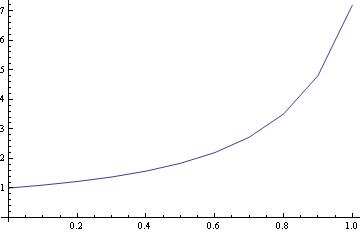
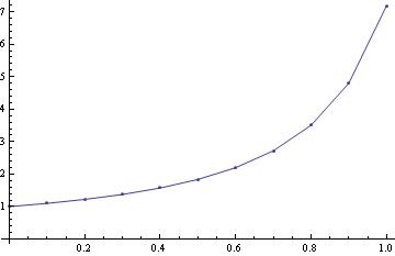
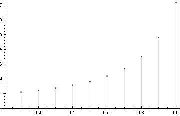
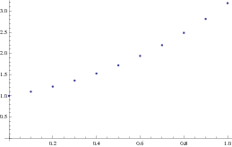
Example: Consider the initial value problem \( y' = x+y, \quad y(0) =1. \)
1.72102}, {0.6, 1.94312}, {0.7, 2.19743}, {0.8, 2.48718}, {0.9, 2.8159}, {1., 3.18748}}
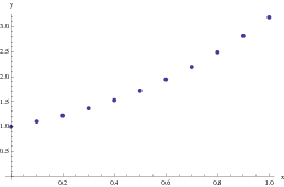
We can plot the output as follows
Or we can plot it as
1.72102}, {0.6, 1.94312}, {0.7, 2.19743}, {0.8, 2.48718}, {0.9,
2.8159}, {1., 3.18748}}
The following code, which uses a slightly different programming
paradigm, implements Euler's method for a system of differential equations:
Module[{t, Y, h = (b - a)/Steps//N, i},
t[0] = a; Y[0] = Y0;
Do[
t[i] = a + i h;
Y[i] = Y[i - 1] + h F[t[i - 1], Y[i - 1]],
{i, 1, n}
];
Table[{t[i], Y[i]}, {i, 0, n}]
]
And the usage message is:
euler::usage = "euler[F, t0, Y0, b, n] gives the numerical solution
to {Y' == F[t, Y], Y[t0] == Y0} over the interval\n
[t0, b] by the n-step Euler's method. The result
is in the form of a table of {t, Y} pairs."
Note that this function uses an exact increment h rather than converting it explicitly to numeric form using Mathematica command N. Of course you can readily change
that or accomplish the corresponding value by giving an approximate
number for one of the endpoints.
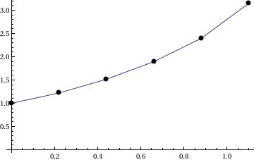
Next we plot the points by joining them with a curve:
Another way without writing a subroutine:
x0 = 0;
y0 = 1;
xend = 1.1;
steps = 5;
h = (xend - x0)/steps // N;
x = x0;
y = y0;
eulerlist = {{x, y}};
For[i = 1, i <= steps, y = f[x, y]*h + y;
x = x + h;
eulerlist = Append[eulerlist, {x, y}]; i++]
Print[eulerlist]
The results can also be visualized by connecting the points:
s = NDSolve[{u'[t] == f[x, u[t]], u[0] == 1}, u[t], {t, 0, 1.1}];
b = Plot[Evaluate[u[x] /. s], {x, 0, 1.1}, PlotStyle -> RGBColor[1, 0, 0]];
Show[a,b]
Next, we illustrate application of Function command:
Module[{h = (t1 - t0)/n // N, tt, yy},
tt[0] = t0; yy[0] = y0;
tt[k_ /; 0 < k < n] := tt[k] = tt[k - 1] + h;
yy[k_ /; 0 < k < n] :=
yy[k] = yy[k - 1] + h f[tt[k - 1], yy[k - 1]];
Table[{tt[k], yy[k]}, {k, 0, n - 1}]
];
Plot[Interpolation[ty][t], {t, 1, 2}]
Here is another steamline of the Euler method (based on Mathematica function), which we demonstrate in
the following
Example: Consider the initial value problem \( y' = y^2 - 3\, x^2 , \quad y(0) =-1. \)
f[x_, y_] := y^2 - 3*x^2
x[1] = 0; y[1] = -1;
h = 0.25; K = IntegerPart[2.5/h]
Do[ { x[i+1] = x[i]+h,
y[i+1] = y[i] +h*f[x[i],y[i]] } , {i,1,K+1} ]
Now we can plot our results, making sure we only refer to values of x and y that we have defined: Now we are going to repeat the problem, but using Mathematica lists format instead. The idea is still the
same---we set a new x value, compute the corresponding y value, and save the two quantities in two
lists. In particular, in a list we are simply storing values; In previously presented code, we were actually
storing rules, which are more complicated to store and evaluate. We start out with just one value in each
list (the initial conditions). Then we use the Append command to add our next pair of values to the list.
pairs = Table[{x[i], y[i]}, {i, 1, K+1}]
plot5 = ListPlot[pairs, Joined -> True, PlotStyle -> {Thickness[0.005], RGBColor[0, 1, 0]}] 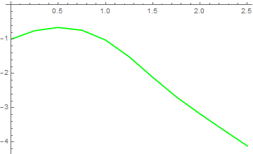
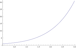
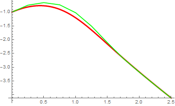
plot1 = Plot[Evaluate[y[x] /. soln], {x, 0, 2.5},
PlotStyle -> {{Thickness[0.008], RGBColor[1, 0, 0]}}];
Show[plot1, plot5]
x = {0.0 };
y = {2.0 };
h = 0.1;
Do [ { x = Append[x,x[[i]]+h],
y = Append[y,y[[i]]+h*f[x[[i]],y[[i]] ] ],
} , {i,1,20} ]
Now we can plot our results:
pairs = Table[ {x[[i]], y[[i]] }, {i,1,21} ]
ListPlot [ pairs, Joined -> True ]
- Atkinson, K., Han, W., Stewart, D., Numerical Solutions of Ordinary Differential Equations, Wiley, 2009.
- Hataue, I., Analysis of ghost numerical solutions of differential equation caused by nonlinear instability, 2012 https://doi.org/10.2514/3.12350
- Yamaguti, M., Ushiki, S., Chaos in numerical analysis of ordinary differential equations, Physica D: Nonlinear Phenomena Volume 3, Issue 3, August 1981, Pages 618-626; https://doi.org/10.1016/0167-2789(81)90044-0
Return to Mathematica page
Return to the main page (APMA0330)
Return to the Part 1 (Plotting)
Return to the Part 2 (First Order ODEs)
Return to the Part 3 (Numerical Methods)
Return to the Part 4 (Second and Higher Order ODEs)
Return to the Part 5 (Series and Recurrences)
Return to the Part 6 (Laplace Transform)
Return to the Part 7 (Boundary Value Problems)