Preface
This section is devoted to an important class of (elementary) functions, called the hyperbolic functions.
Return to computing page for the second course APMA0340
Return to Mathematica tutorial for the first course APMA0330
Return to Mathematica tutorial for the second course APMA0340
Return to the main page for the course APMA0330
Return to the main page for the course APMA0340
Return to Part VII of the course APMA0330
Glossary
Hyperbolic Functions
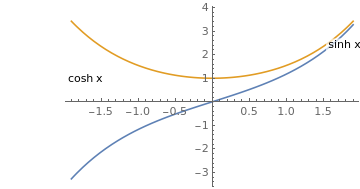
Two particular combinations of exponential functions appear frquently in many applications that it has been worth-while to use special symbols for those combinations. The hyperbolic sine of a variable x, written sinhx (or shx), is defined by
\[
\sinh x = \frac{1}{2}\, e^x - \frac{1}{2}\, e^{-x} ;
\]
the hyperbolic cosine of x, written coshx (or chx). is defined by
\[
\cosh x = \frac{1}{2}\, e^x + \frac{1}{2}\, e^{-x} .
\]
Mathematica has dedicated commands for these functions: Sinh[x] and Cosh[x]. Hyperbolic functions were introduced in the 1760s independently by Vincenzo Riccati and Johann Heinrich Lambert. The hyperbolic functions are related to regular trigonometric functions due to Euler's formulas:
\[
\sin x = \frac{1}{2{\bf j}}\, e^{{\bf j} \,x} - \frac{1}{2{\bf j}}\, e^{-{\bf j} \,x} , \qquad \cos x = \frac{1}{2}\, e^{{\bf j} \,x} + \frac{1}{2}\, e^{-{\bf j} \,x} , \quad {\bf j}^2 =-1.
\]
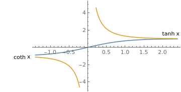
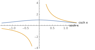
Four more hyperbolic functions are
\begin{align*}
\tanh x &= \frac{\sinh x}{\cosh x} , \qquad \sech x = \frac{1}{\cosh x} ,
\\
\csch x &= \frac{1}{\sinh x} , \qquad \coth x = \frac{\cosh x}{\sinh x} .
\end{align*}
Plot[{Sinh[x], Cosh[x]}, {x, -1.9, 1.9},
PlotLabels -> Placed[{"sinh x", "cosh x"}, {Scaled[1], Before}]]
Plot[{Tanh[x], Coth[x]}, {x, -1.4, 1.4},
PlotLabels -> Placed[{"tanh x", "coth x"}, {Scaled[1], Before}]]
Plot[{Sech[x], Csch[x]}, {x, -1.4, 1.4},
PlotLabels -> Placed[{"sech x", "csch x"}, {Scaled[1], After}]]
|
|
|
\[
\cosh^2 x - \sinh^2 x =1,
\]
an identity similar to the well-known identity cos²x + sin²x = 1 in circular trigonometry. Derivative formulas are also similar:
\[
\frac{\text d}{{\text d}x}\,\sinh x = \cosh x , \qquad \frac{\text d}{{\text d}x}\,\cosh x = \sinh x.
\]
From above graph, we see that coshx and sinhx satisfy the following relations
\begin{align*}
\cosh \left( x+y \right) &= \cosh x\,\cosh y + \sinh x\,\sinh y, \qquad
\cosh \left( x-y \right) = \cosh x\,\cosh y - \sinh x\,\sinh y,
\\
\sinh \left( x+y \right) &= \sinh x\,\cosh y + \cosh x \,\sinh y , \qquad
\sinh \left( x-y \right) = \sinh x\,\cosh y - \cosh x\,\sinh y,
\\
\sinh^2 y &= \frac{1}{2} \left( \cosh 2y - 1 \right) , \qquad \cosh^2 y = \frac{1}{2} \left( \cosh 2y +1 \right) ,
\\
\cosh 2y &= \cosh^2 y + \sinh^2 y = 2\,\cosh^2 y -1 = 2\,\sinh^2 y +1 ,
\\
\sinh 2y &= 2\,\sinh y\,\cosh y ,
\\
\tanh \left( x+y \right) &= \frac{\tanh x + \tanh y}{1+ \tanh x\,\tanh y} .
\end{align*}
Return to Mathematica page
Return to the main page (APMA0330)
Return to the Part 1 (Plotting)
Return to the Part 2 (First Order ODEs)
Return to the Part 3 (Numerical Methods)
Return to the Part 4 (Second and Higher Order ODEs)
Return to the Part 5 (Series and Recurrences)
Return to the Part 6 (Laplace Transform)
Return to the Part 7 (Boundary Value Problems)