Return to computing page for the second course APMA0340
Return to Mathematica tutorial for the first course APMA0330
Return to Mathematica tutorial for the second course APMA0340
Return to the main page for the course APMA0330
Return to the main page for the course APMA0340
Return to Part III of the course APMA0330
Glossary
Backward Euler method
Suppose that we wish to numerically solve the initial value problem
|
\[
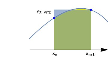
y_{n+1} = y_n + h\, f(x_{n+1}, y_{n+1}) , \qquad y_0 = y(0), \qquad n=0,1,2,\ldots .
\]
|
|---|
 |
curve=Plot[x-Exp[x-0.05]+1.5,{x,-1.0,0.7},PlotStyle->Thick,Axes->False,Epilog->{Blue,PointSize@Large,Point[{{-0.5,0.42},{0.25,0.53}}]},PlotRange->{{-1.6,0.6},{-0.22,0.66}}];
line=ListLinePlot[{{-0.5,0.53},{0.25,0.53}},Filling->Bottom,FillingStyle->Opacity[0.6]]; curve2=Plot[x-Exp[x-0.05]+1.5,{x,-0.5,0.25},PlotStyle->Thick,Axes->False,PlotRange->{{-1.6,0.6},{0.0,0.66}},Filling->Bottom,FillingStyle->Yellow]; ar1=Graphics[{Black,Arrowheads[0.07],Arrow[{{-1.0,0.0},{0.6,0.0}}]}]; t1=Graphics[Text[Style["f(t, y(t))",FontSize->12],{-0.7,0.5}]]; xn = Graphics[ Text[Style[Subscript["x", "n"], FontSize -> 12, FontColor -> Black, Bold], {-0.48, -0.05}]]; xn1 = Graphics[ Text[Style[Subscript["x", "n+1"], FontSize -> 12, FontColor -> Black, Bold], {0.24, -0.05}]]; Show[curve,curve2,line,ar1,t1,xn,xn1] |
The backward Euler formula is an implicit one-step numerical method for solving initial value problems for first order differential equations. It requires more effort to solve for yn+1 than Euler's rule because yn+1 appears inside f. The backward Euler method is an implicit method: the new approximation yn+1 appears on both sides of the equation, and thus the method needs to solve an algebraic equation for the unknown yn+1. Frequently a numerical method like Newton's that we consider in the section must be used to solve for yn+1. The backward Euler method is also a one-step method similar to the forward Euler rule.
Here is a Mathematica code to perform the backward Euler rule:
Block[{xold = x0, yold = y0, sollist = {{x0, y0}}, h},
h = N[(xn - x0)/steps];
Do[xnew = xold + h;
s = FindRoot[ynew == yold + h*f[xnew, ynew], {ynew, yold}];
yn = ynew /. s;
sollist = Append[sollist, {xnew, yn}];
xold = xnew; yold = yn, {steps}];
Return[sollist]]
backeuler[{0, 1}, {1/2}, 10]
NSolve has to spend time to compute all roots to the equation (which can be computationally
expensive). FindRoot does a pretty fast search looking for only a single root, so it is quick
for complex equations.
If you care about all possible roots, or if you have no clue where the roots of the equation may be,
FindRoot is a terrible choice. If you only care about a single root and have a rough idea of
where it might be, though, FindRoot will find it quickly. Therefore, we use only this command in the backward Euler formula.
Example: Consider the initial value problem for the linear equation
| n | xn | yn | Exact solution | Absolute error |
|---|---|---|---|---|
| 1 | 0.1 | |||
| 2 | 0.2 | |||
| 3 | 0.3 | |||
| 4 | 0.4 | |||
| 5 | 0.5 | |||
| 6 | 0.6 | |||
| 7 | 0.7 | |||
| 8 | 0.8 | |||
| 9 | 0.9 | |||
| 10 | 1.0 |
Example: Consider the initial value problem for the logistic equation
| n | xn | yn | Exact solution | Absolute error |
|---|---|---|---|---|
| 1 | 0.1 | |||
| 2 | 0.2 | |||
| 3 | 0.3 | |||
| 4 | 0.4 | |||
| 5 | 0.5 | |||
| 6 | 0.6 | |||
| 7 | 0.7 | |||
| 8 | 0.8 | |||
| 9 | 0.9 | |||
| 10 | 1.0 |
Example: Consider the initial value problem \( y'= 1/(3x-2y+1),\quad y(0)=0 \)
| n | xn | yn | Exact solution | Absolute error |
|---|---|---|---|---|
| 1 | 0.1 | |||
| 2 | 0.2 | |||
| 3 | 0.3 | |||
| 4 | 0.4 | |||
| 5 | 0.5 | |||
| 6 | 0.6 | |||
| 7 | 0.7 | |||
| 8 | 0.8 | |||
| 9 | 0.9 | |||
| 10 | 1.0 |
Example: Consider the following initial value problem:
h = 0.1; (* step size *)
t[0] = 0.; (* starting value of the independent value *)
M = Round[0.5/h]; (* number of points to reach the final destination, in our case it is 0.5 *)
toler = h; (* define the tolerance *)
Do[
t[n + 1] = t[n] + h;
eqn = (z == y[n] + h (z^3 - 3 t[n + 1]) );
ans = z /. NSolve[eqn, z, Reals];
indlist = {};
toler = h;
While[ Length[indlist] == 0,
toler = toler*2.;
indlist = Flatten[Position[Map[(Abs[y[n] - #] < toler) &, ans], True]];
];
ind = indlist[[1]];
y[n + 1] = ans[[ind]];
, {n, 0, M}]
Then we plot the solution:
y[M]
t[M]
| n | xn | yn | Exact solution | Absolute error |
|---|---|---|---|---|
| 1 | 0.1 | |||
| 2 | 0.2 | |||
| 3 | 0.3 | |||
| 4 | 0.4 | |||
| 5 | 0.5 | |||
| 6 | 0.6 | |||
| 7 | 0.7 | |||
| 8 | 0.8 | |||
| 9 | 0.9 | |||
| 10 | 1.0 |
Central Difference Scheme
Example: We consider the following initial value problem for the Riccati equation
| n | xn | yn | Exact solution | Absolute error |
|---|---|---|---|---|
| 1 | 0.1 | |||
| 2 | 0.2 | |||
| 3 | 0.3 | |||
| 4 | 0.4 | |||
| 5 | 0.5 | |||
| 6 | 0.6 | |||
| 7 | 0.7 | |||
| 8 | 0.8 | |||
| 9 | 0.9 | |||
| 10 | 1.0 |
Nonstandard Euler Methods
Let ϕ be a real-valued function on ℝ that satisfies the property:
- nonstandard explicit Euler method given by
\[ \frac{y_{k+1} - y_k}{\phi (hq)/q} = f(y_k ), \qquad y_0 = y(0), \quad k=0,1,2,\ldots . \]
- nonstandard implicit Euler method given by
\[ \frac{y_{k+1} - y_k}{\phi (hq)/q} = f(y_{k+1} ), \qquad y_0 = y(0), \quad k=0,1,2,\ldots . \]
Example: Consider the initial value problem
| n | xn | yn | Exact solution | Absolute error |
|---|---|---|---|---|
| 1 | 0.1 | |||
| 2 | 0.2 | |||
| 3 | 0.3 | |||
| 4 | 0.4 | |||
| 5 | 0.5 | |||
| 6 | 0.6 | |||
| 7 | 0.7 | |||
| 8 | 0.8 | |||
| 9 | 0.9 | |||
| 10 | 1.0 |
| n | xn | yn | Exact solution | Absolute error |
|---|---|---|---|---|
| 1 | 0.1 | |||
| 2 | 0.2 | |||
| 3 | 0.3 | |||
| 4 | 0.4 | |||
| 5 | 0.5 | |||
| 6 | 0.6 | |||
| 7 | 0.7 | |||
| 8 | 0.8 | |||
| 9 | 0.9 | |||
| 10 | 1.0 |
| n | xn | yn | Exact solution | Absolute error |
|---|---|---|---|---|
| 1 | 0.1 | |||
| 2 | 0.2 | |||
| 3 | 0.3 | |||
| 4 | 0.4 | |||
| 5 | 0.5 | |||
| 6 | 0.6 | |||
| 7 | 0.7 | |||
| 8 | 0.8 | |||
| 9 | 0.9 | |||
| 10 | 1.0 |
Return to Mathematica page
Return to the main page (APMA0330)
Return to the Part 1 (Plotting)
Return to the Part 2 (First Order ODEs)
Return to the Part 3 (Numerical Methods)
Return to the Part 4 (Second and Higher Order ODEs)
Return to the Part 5 (Series and Recurrences)
Return to the Part 6 (Laplace Transform)
Return to the Part 7 (Boundary Value Problems)