Preface


A function μ is called an integrating factor if and only if multiplication by it reduces the differential equation \( M(x,y)\,{\text d}x + N(x,y)\,{\text d} y =0 \) to an exact equation. Although Alexis Clairaut was the first to discover integrating factors, the fundamental conception of this technique iis due to Leonhard Euler, who set up classes of equations that admit integrating factors.
Return to computing page for the first course APMA0330
Return to computing page for the second course APMA0340
Return to Mathematica tutorial for the second course APMA0340
Return to the main page for the course APMA0330
Return to the main page for the course APMA0340
Return to Part II of the course APMA0330

Integrating Factors


In many cases, a differential equation of first order
\[ M(x,y)\,{\text d}x + N(x,y)\,{\text d}y =0 \]
can be converted into an exact equation by multiplying through appropriate function. Correspondingly, a function \( \mu = \mu (x,y) \) is called an integrating factor if, upon multiplication the above equation by μ, we obtain an exact equation. In other words, μ is an integrating factor if and only if
\[ \frac{\partial}{\partial y} \left( \mu \,M(x,y)\right) = \frac{\partial}{\partial x} \left( \mu \,N(x,y)\right) . \]
This is especially useful in thermodynamics where temperature becomes the integrating factor that makes entropy an exact differential.
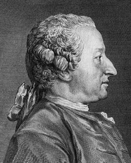
Alexis Clairaut

The integrating factor method was introduced by the French mathematician, astronomer, and geophysicist Alexis Claude Clairaut (1713--1765). He was a prominent Newtonian follower whose work helped to establish the validity of the principles and results that Sir Iaac Newton had outlined in the Principia of 1687. Clairaut was one of the key figures in the expedition to Lapland that helped to confirm Newton's theory for the figure of the Earth. In that context, Clairaut worked out a mathematical result now known as "Clairaut's theorem". He also tackled the gravitational three-body problem, being the first to obtain a satisfactory result for the apsidal precession (rotation of the orbit of a celestial body) of the Moon's orbit. Clairaut published some important work during the period 1733 to 1743. He wrote a paper in 1733 on the calculus of variations, and in the same year he published on the geodesics of quadrics of rotation. The following year Clairaut studied the differential equations now known as Clairaut's differential equations, and introduced a singular solution in addition to the general integral of the equations. In 1739 and 1740, he published further work on the integral calculus, proving the existence of integrating factors for solving first order differential equations. In 1742, Clairaut published an important work on dynamics. Clairaut was unmarried, and known for leading an active social life.

Using simplified notations μx and μy for partial derivatives with respect to x and y, respectively, we rewrite the above partial differential equation as

\[ \mu_x N(x,y) - \mu_y M(x,y) = \mu \left( M_y - N_x \right) . \]
Upon division by μ, we get
\[ \frac{\mu_x}{\mu} \, N(x,y) - \frac{\mu_y}{\mu}\, M(x,y) = M_y - N_x . \]
Actually, the conversion of a differential equation into an exact equation using an integrating factor is extremely general. Unfortunately, there is no systematic way to solve the above partial differential equation with respect to μ. There are known particular classes when it is possible, and we consider some of them. It is also sometimes convenient to reduce the partial differential equation for logarithm of μ. Let
\[ G(x,y) = \frac{\mu_x}{\mu} \qquad\mbox{and}\qquad F(x,y) = \frac{\mu_y}{\mu} . \]
Since \( \frac{\partial}{\partial x}\, \ln \mu = G(x,y) \) and \( \frac{\partial}{\partial y}\, \ln \mu = F(x,y) , \) we find
\[ \mu (x,y) = e^{\int G(x,y)\,{\text d} x} \,e^{\int F(x,y)\,{\text d} y} , \]
where F and G are solutions of the algebraic equation
\[ G(x,y) \,N(x,y) - F(x,y)\, M(x,y) = M_y - N_x . \]

We start with two simple (but very important) classes when an integrating factor depends on only one variable.

  • Suppose that an integrating factor depends only on the independent variable only. Then \( \mu = \mu (x) \) satisfies the differential equation
    \[ \frac{\partial}{\partial y} \left( \mu \,M(x,y)\right) = \frac{\partial}{\partial x} \left( \mu \,N(x,y)\right) \qquad \Longleftrightarrow \qquad \mu \, \frac{\partial M(x,y)}{\partial y} = \frac{{\text d} \mu}{{\text d} x} \, N(x,y) + \mu \, \frac{\partial N(x,y)}{\partial x} . \]
    Then we get the equation
    \[ \frac{1}{\mu} \,\frac{{\text d} \mu}{{\text d} x} = \frac{M_y - N_x}{N(x,y)} \qquad \mbox{must be a function of $x$ only} \]
    because the left-hand side is a function of x. In this case, variable are separated and upon integration, we obtain
    \[ \mu (x) = \exp \left\{ \int \frac{M_y - N_x}{N(x,y)} \, {\text d} x \right\} . \]
  • Suppose that an integrating factor depends only on the dependent variable only. Then \( \mu = \mu (y) \) satisfies the differential equation
    \[ \frac{\partial}{\partial y} \left( \mu \,M(x,y)\right) = \frac{\partial}{\partial x} \left( \mu \,N(x,y)\right) \qquad \Longleftrightarrow \qquad \mu \, \frac{\partial M(x,y)}{\partial y} + \frac{{\text d} \mu}{{\text d} y} \, M(x,y) = \mu \, \frac{\partial N(x,y)}{\partial x} . \]
    Then we get the equation
    \[ \frac{1}{\mu} \,\frac{{\text d} \mu}{{\text d} y} = -\frac{M_y - N_x}{M(x,y)} \qquad \mbox{must be a function of $y$ only} \]
    because the left-hand side is a function of y. In this case, variable are separated and upon integration, we obtain
    \[ \mu (y) = \exp \left\{ -\int \frac{M_y - N_x}{M(x,y)} \, {\text d} y \right\} . \]
An integrating factor is not unique, as the following example shows.

Example: Solve the equation

\[ \left( 3xy + y^2 \right) {\text d}x + \left( x^2 + xy \right) {\text d}y =0 . \]

Solution. With \( M(x,y) = 3xy + y^2 , \quad N(x,y) = x^2 + xy , \) we see that \( M_y = 3x + 2y \ne N_x = 2x +y . \) Therefore, the given equation is not exact. Since the ratio

\[ \frac{M_y - N_x}{N} = \frac{x+y}{x^2 + xy} = \frac{1}{x} \]
is a function of x, there exists an integrating factor \( \mu = \mu (x) = x . \) Multiplication by μ reduces the given differential equation to an exact one:
\[ \left( 3x^2 y + x\,y^2 \right) {\text d}x + \left( x^3 + x^2 y \right) {\text d}y =0 . \]
Indeed, with new coefficients \( M(x,y) = 3x^2 y + x\,y^2 , \quad N(x,y) = x^3 + x^2 y , \) we have \( M_y = 3x^2 + 2xy = N_x = 3x^2 + 2xy . \) Therefore, the given equation is exact. Then there exists a potential function ψ such that
\[ \frac{\partial \psi}{\partial x} = M(x,y) = 3x^2 y + x\,y^2 , \qquad \frac{\partial \psi}{\partial y} = N(x,y) = x^3 + x^2 y . \]
Integrating the former, we get \( \psi (x,y) = x^3 y + \frac{1}{2}\, x^2 y^2 + h(y) \) for some (unknown) function h(y). Differentiating ψ with respect to y and equating the result to N, we get
\[ \frac{\partial \psi}{\partial y} = 3x^2 y + x\,y^2 + h' (y) = N(x,y) = 3x^2 y + x\,y^2 \qquad \Longrightarrow \qquad h' =0 . \]
So h(y) is a constant, which we drop. Therefore, we obtain the general solution in implicit form:
\[ \psi (x,y) = C \qquad \Longleftrightarrow \qquad x^3 y + \frac{1}{2}\, x^2 y^2 = C , \]
for some constant C.

Note that the function

\[ \mu (x,y) = \frac{1}{xy\left( 2x+y \right)} \]
can also be used as an integrating factor. ■

Example: Solve the equation

\[ \left( 5x^4 y^4 + 2y\, e^{2x} + y^2 \cos (xy) \right) {\text d}x + \left( 3x^5 y^3 + xy \, \cos (xy) \right) {\text d}y =0 . \]

Solution. With \( M(x,y) = 5x^4 y^4 + 2y\, e^{2x} + y^2 \cos (xy) , \quad N(x,y) = 3x^5 y^3 + xy \, \cos (xy) , \) we see that \( M_y = 20x^4 y^3 + 2\, e^{2x} + 2y \, \cos (xy) - xy^2 \sin (xy) \ne N_x = 15 x^4 y^3 + y\,\cos (xy) - xy^2 \sin (xy) . \) Therefore, the given equation is not exact, but the ratio

\[ \frac{M_y - N_x}{M} = \frac{5x^4 y^3 + 2\, e^{2x} +y\,\cos (xy)}{5x^4 y^4 + 2y\, e^{2x} +y^2\,\cos (xy)} = \frac{1}{y} \]
is a function of y only. Therefore, there exists an integrating factor as a factor of y:
\[ \mu (y) = \exp \left\{ -\frac{M_y - N_x}{M}\, {\text d}y \right\} = \frac{1}{y} . \]
Multiplying by μ(y), we obtain an exact equation, which upon integrating, we obtain the general solution:
\[ \psi (x,y) = C \qquad \Longleftrightarrow \qquad x^5 y^3 + e^{2x} + \sin (xy) =C , \]
where C is an arbitrary constant. ■

In some instances, an integrating factor of a differential equation can be found by inspection, a process based on ingenuity and experience. We present a list of integrating factors that may be helpful in solving differential equations.

With the Use the  
combination integrating factor To obtain the exact differential
\( y\,{\text d}x + x\,{\text d}y \) \( \displaystyle \begin{split} \frac{1}{xy} \\ \frac{1}{(xy)^n} , \ n \ne 1 \end{split} \) \( \displaystyle \begin{split} \frac{y\,{\text d}x + x\,{\text d}y}{xy} = {\text d}(\ln xy) \\ \frac{y\,{\text d}x + x\,{\text d}y}{(xy)^n} = -{\text d} \left( \frac{1}{(n-1) (xy)^{n-1}} \right) \end{split} \)
\( x\,{\text d}x + y\,{\text d}y \) \( \displaystyle \begin{split} \frac{1}{x^2 + y^2} \\ \frac{1}{(x^2 + y^2 )^n} , \ n\neq 1 \end{split} \) \( \displaystyle \begin{split} \frac{x\,{\text d}x + y\,{\text d}y}{x^2 + y^2} = \frac{1}{2} \, {\text d}\left( \ln (x^2 + y^2 ) \right) \\ \frac{x\,{\text d}x + y\,{\text d}y}{(x^2 + y^2 )^n} = -\frac{1}{2} \,{\text d}\left( \frac{1}{(n-1) (x^2 + y^2 )^{n-1}} \right) \end{split} \)
\( y\,{\text d}x - x\,{\text d}y \) \( \displaystyle \begin{split} \frac{1}{y^2} \\ \frac{1}{x^2} \\ \frac{1}{xy} \\ \frac{1}{x^2 + y^2} \end{split} \) \( \displaystyle \begin{split} \frac{y\,{\text d}x - x\,{\text d}y}{y^2} = {\text d}\left( \frac{x}{y} \right) \\ \frac{y\,{\text d}x - x\,{\text d}y}{x^2} = -{\text d}\left( \frac{y}{x} \right) \\ \frac{y\,{\text d}x - x\,{\text d}y}{xy} = {\text d}\left( \ln\frac{x}{y} \right) \\ \frac{y\,{\text d}x - x\,{\text d}y}{x^2 + y^2} = {\text d}\left( \arctan \frac{x}{y} \right) \end{split} \)

Example: Solve the equation

\[ \left( 4x^4 y + y\right) {\text d}x + x\,{\text d}y =0 . \]

Solution. First, we rewrite the equation as

\[ 4x^4 y \,{\text d}x + \left( y\,{\text d}x + x\,{\text d}y \right) =0 . \]
The table suggests that we try μ = (xy)-1 as an integrating factor. Multiplying by μ gives
\[ 4x^3 \,{\text d}x + \frac{y\,{\text d}x + x\,{\text d}y}{xy} =0 \qquad\mbox{or} \qquad {\text d}x^4 + {\text d} \left( \ln \, xy \right) =0, \]
and the general solution is obtained by just integration: \( x^4 + \ln \, xy = C , \) with some constant C.

Example: Solve the equation

\[ (3xy^4 + y)\,{\text d}x + (x^2 y^3 -x)\,{\text d}y =0 . \]

Solution. We consider the group \( y\,{\text d}x - x\,{\text d}y , \) which is not exact, but becomes so after division by xy (\( x\ne 0 \mbox{ and } y\ne 0 \) ). Then the given equation is reduced to

\[ 3y^3\,{\text d}x + xy^2 \,{\text d}y + \frac{y\,{\text d}x -x\,{\text d}y}{xy} =0 \qquad \Longrightarrow \qquad 3y^3 \,{\text d}x + xy^2 \,{\text d}y + {\text d}\,\ln \left( \frac{x}{y} \right) =0. \]
The last term is now exact and will remain exact when multiplied by any function of x/y. Therefore, we let z=x/y and choose φ(z) in such a way that \( \phi (z) \left( 3y^3 \,{\text d}x + xy^2 \,{\text d}y \right) \) is exact. Using relations \( \partial \phi /\partial x = \phi' (z) /y \) and \( \partial \phi /\partial y = -\phi' (z) x/ y^2 , \) we evaluate partial derivatives
\[ \frac{\partial}{\partial y} \left( \phi (z)\,3y^3 \right) = - \phi' (z)\,\frac{x}{y^2}\,3y^3 + \phi (z)\, 9y^2 \qquad\mbox{and}\qquad \frac{\partial}{\partial x} \left( \phi (z)\,xy^2 \right) = \phi' (z)\,\frac{1}{y} \,xy^2 + \phi \,y^2 . \]
For φ(z) to be an integrating factor, we need to choose it so that these two partial derivatives are equal:
\[ - 3\phi' (z) \,xy + 9y^2 \,\phi (z) = xy\,\phi' (z) +y^2 \,\phi \qquad \Longrightarrow \qquad \phi' (z) = \phi (z) \,\frac{2y}{x} = 2\phi (z) /z. \]
Solving this equation for φ, we get the integrating factor \( \phi (z) =z^2 = x^2 /y^2 . \) Multiplying by it, we obtain the exact equation: \[ \left( 3x^2 y + \frac{x}{y^2} \right) {\text d}x + \left( x^3 - \frac{x^2}{y^3} \right) {\text d}y =0 \qquad \Longrightarrow \qquad {\text d} \left( x^3 y + \frac{x^2}{2y^2} \right) =0 . \]
Hence, the general solution is \( x^3 y + \frac{x^2}{2y^2} =C, \) where C is an arbitrary constant. ■

A function of two variables g(x,y) is called homogeneous of degree r if \( g(\lambda x , \lambda y ) = \lambda^r g(x,y) \) for any nonzero constant λ and some real number r (possibly zero). If M(x,y) and N(x,y) are homogeneous functions of the same degree, then an integrating factor

\begin{equation} \label{E15.7} \mu (x,y) = \frac{1}{x M(x,y) + y N(x,y)} \end{equation}
reduces \( M(x,y)\,{\text d}x + N(x,y) \,{\text d}y =0 \) to an exact equation. In this case it is also possible to reduce \( M(x,y)\,{\text d}x + N(x,y) \,{\text d}y =0 \) to the equation
\[ \frac{{\text d}y}{{\text d}x} = -\frac{M(x,y)}{N(x,y)} \]
with a homogeneous right-hand side function, that is, \( \frac{M(\lambda x,\lambda y)}{N(\lambda x, \lambda y)} =\frac{\lambda^r \,M(x,y)}{\lambda^r \,N(x,y)} = \frac{M(x,y)}{N(x,y)} . \)

Example: Consider the differential equation

\[ xy\,{\text d}x+( x^2 + y^2 )\,{\text d}y =0. \]
Since \( M(x,y)=xy \) and \( N(x,y)= x^2 + y^2 \) are homogeneous functions of the second degree, we choose an integrating factor in the form \( \mu (x,y) = \frac{1}{x M(x,y) + y N(x,y)} \) to obtain
\[ \mu (x,y) = \frac{1}{x^2 y + y( x^2 + y^2 )} = \frac{1}{y( 2 x^2 + y^2 )} . \]
Multiplication of the given equation by μ(x,y) leads to an exact differential equation \( \tilde{M} (x,y) \,{\text d}x + \tilde{N} (x,y)\,{\text d}y =0 \) with
\[ \tilde{M} (x,y) = \frac{x}{ 2 x^2 + y^2} , \quad \tilde{N} (x,y) = \frac{x^2 + y^2}{y (2 x^2 + y^2 )} \]
since \( \tilde{M}_y = \tilde{N}_x . \) Therefore, there exists a function ψ(x,y) such that
\[ {\text d}\psi (x,y) = \tilde{M} (x,y) \,{\text d}x + \tilde{N} (x,y)\,{\text d}y =0 . \]
Integrating the equation \( \displaystyle \frac{\partial \psi}{\partial x} = \frac{x}{ 2 x^2 + y^2} , \) we obtain
\[ \psi (x,y) = \frac{1}{4}\,\ln | 2 x^2 + y^2 | + h(y) \]
with some unknown function h(y). Equating ψy, the partial derivative of ψ(x,y) with respect to y, to \( \tilde{N} (x,y) \) yields
\[ \frac{\partial \psi}{\partial y} = \frac{1}{2} \,\frac{y}{ 2 x^2 + y^2} + h' (y) =\frac{x^2 + y^2}{y (2 x^2 + y^2 )} . \]
From the last equation we have \ \( h' (y) = 1/(2y) \) \ and\ \( h(y) = 0.5 \ln y . \) Hence, the potential function ψ is
\[ \psi (x,y) = \frac{1}{4}\,\ln ( 2 x^2 + y^2 ) + \frac{1}{2}\,\ln |y| = \frac{1}{4}\,\ln ( 2 x^2 y^2+ y^4) . \]
We can also rewrite the equation in the form
\[ \frac{{\text d}y}{{\text d}x} = -\frac{xy}{ x^2 + y^2 } . \]
By setting y=vx, we obtain \( x\, v' + v = - v/(1+ v^2 ) . \) Separation of variables yields
\[ \frac{1+ v^2}{v(2+ v^2 )} \,{\text d}v = - \frac{{\text d}x}{x} . \]
Integration shows that \( x^4 v^2 ( 2 + v^2 ) = C \) since
\[ \frac{1+ v^2}{v(2+ v^2 )} = \frac{1}{2} \left[ \frac{1}{v} + \frac{v}{2+ v^2} \right] . \]
Substituting v=y/x yields the same general solution as before: \( \psi (x,y) \equiv y^2 ( 2 x^2 + y^2 ) = C. \)

The integrating factor

\begin{equation} \label{E15.8} \mu (x,y) = \frac{1}{xy [ p(xy) - q(xy) ]} %\eqno{(5.8)}$$ \end{equation}
reduces \( M(x,y)\,{\text d}x + N(x,y) \,{\text d}y =0 \) to an exact differential equation if
\begin{equation} \label{E15.8a} M(x,y) = y\,p(xy) \quad \mbox{and} \quad N(x,y) = x\,q(xy), \quad p(xy) \neq q(xy)\, . \end{equation}

Example: The differential equation

\[ x y^2\,{\text d}x + x^3 y^2 \,{\text d}y =0 \]
is a differential equation of the form \( M(x,y)\,{\text d}x + N(x,y) \,{\text d}y =0 , \) with \( M(x,y) = y\,p(xy) , \quad N(x,y) = x\,q(xy) , \) where p(z) = z, q(z) = z². Therefore, this equation can be reduced to an exact equation with the integrating factor \( \mu (x,y) = \frac{1}{xy [ p(xy) - q(xy) ]}; \) namely,
\[ \mu (x,y) = \frac{1}{xy (xy - x^2 y^2 )} = \frac{1}{x^2 y^2 (1-xy)} . \]
Multiplication of the given equation by μ(x,y) yields
\[ \frac{{\text d}x}{x(1-xy)} + \frac{x\,{\text d}y}{1-xy} =0 . \]
The last equation is an exact differential equation with the potential function &psi(x,y). Integration gives
\[ \psi (x,y) = \ln |x| - \ln |1-xy| = \ln \left\vert \frac{x}{1-xy} \right\vert . \]

Integrating factors of the form \( \mu = \mu (\omega (x,y)) \)


Suppose that for a given differential equation \( M(x,y)\,{\text d}x + N(x,y)\,{\text d}y =0 \) there exists an integrating factor of the form \( \mu = \mu (\omega (x,y)) \) for some function ω(x,y) of two variables. From equation \( \left( \mu\,M \right)_y = \left( \mu\,N \right)_x , \) we obtain

\[ N \,\frac{d\mu}{d\omega} \cdot \frac{\partial\omega}{\partial x} - M\, \frac{d\mu}{d\omega}\cdot\frac{\partial\omega}{\partial y} = \left( \frac{\partial M}{\partial y} - \frac{\partial N}{\partial x} \right) \,\mu (\omega ) \quad \mbox{or} \quad \frac{\mu'}{\mu} = \dfrac{\dfrac{\partial M}{\partial y} - \dfrac{\partial N}{\partial x} }{N \dfrac{\partial\omega}{\partial x} - M \dfrac{\partial\omega}{\partial y}} . \]
Thus, if
\begin{equation} \label{E15.9} \dfrac{\dfrac{\partial M}{\partial y} - \dfrac{\partial N}{\partial x} }{N \dfrac{\partial\omega}{\partial x} - M \dfrac{\partial\omega}{\partial y}} = \chi (\omega ) %\eqno{(5.9)} \end{equation}
is a function of ω alone, we can find an integrating factor explicitly:
\begin{equation} \label{E15.10} \mu (x,y) = \exp \left\{ \int \chi (\omega )\,d\omega \right \} . \end{equation}


Return to Mathematica page
Return to the main page (APMA0330)
Return to the Part 1 (Plotting)
Return to the Part 2 (First Order ODEs)
Return to the Part 3 (Numerical Methods)
Return to the Part 4 (Second and Higher Order ODEs)
Return to the Part 5 (Series and Recurrences)
Return to the Part 6 (Laplace Transform)
Return to the Part 7 (Boundary Value Problems)