Preface
This section discusses numerical solutions to the differential equations of order larger than one.
Return to computing page for the second course APMA0340
Return to Mathematica tutorial for the second course APMA0340
Return to the main page for the course APMA0330
Return to the main page for the course APMA0340
Return to Part IV of the course APMA0330
Glossary
Numerical Solutions
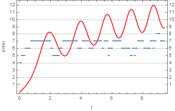
The order of a numerical method used in NDSolve is a variable. Based on What's inside InterpolatingFunction[{{1., 4.}}, <>]?, the following shows the order at each step. Note that the first few steps are NDSolve getting its bearings before the first Adams steps (order 4). With InterpolationOrder -> All, the solution is returned with local series for the Adams steps. Their length should be one more than the order of the step, I think. The documentation says it should be the "same order as the underlying method used."
Example. let use Adams method to solve numerically the following initial value problem
Method -> "Adams", InterpolationOrder -> All];
adamsifn = x /. First@adamssol
(*ifn[[4]]= local series coefficients*)
Transpose@{Flatten@adamsifn["Grid"],
Rescale[#, MinMax[#], {0, 12}] &@adamsifn["ValuesOnGrid"]}}, Joined -> {False, True},
Frame -> True, FrameLabel -> {"t", "order"}, FrameTicks -> {Automatic, Range@12},
GridLines -> {None, Automatic}, PlotStyle -> {Thick, Red}]
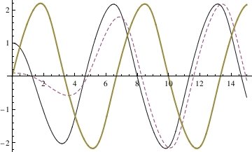
Example: Rayleigh's equation is a non-linear equation
\[ x'' + \mu \left( x^2 -1\right) x +x =0 , \]
that arises in the study of the motion of a violin string. We plot three solutions subject to three different initial conditions:
x'[0] == 0}, x[t], {t, 0, 15}]
Plot[Evaluate[x[t] /. {numsol, numsol2, numsol3}], {t, 0, 15},
PlotStyle -> {GrayLevel[0.1], Dashed, Thick}]

To identify each graph, it is helpful to use PlotLegend option:
PlotLegends -> Automatic]

PlotLegends -> {"IC: x(0)=1, x'(0)=0", "IC: x(0)=0.1, x'(0)=0", "IC: x(0)=0, x'(0)=2"}]
Example: Consider the second-order nonlinear differential equation with the product of the derivative and a sinusoidal nonlinearity of the solution
- Quarteroni, Alfio, Numerical Models for Differential Problems, , Springer International Publishing, 2017, New York, ISBN: 978-3-319-49316-9; doi: 10.1007/978-3-319-49316-9
- Schwalbe, Dan, and Wagon, Stan, VisualDSolve, Springer-Verlag, New York, 1997, ISBN: 978-1-4612-7473-5
Return to Mathematica page
Return to the main page (APMA0330)
Return to the Part 1 (Plotting)
Return to the Part 2 (First Order ODEs)
Return to the Part 3 (Numerical Methods)
Return to the Part 4 (Second and Higher Order ODEs)
Return to the Part 5 (Series and Recurrences)
Return to the Part 6 (Laplace Transform)