Return to computing page for the first course APMA0330
Return to computing page for the second course APMA0340
Return to Mathematica tutorial for the second course APMA0340
Return to the main page for the course APMA0330
Return to the main page for the course APMA0340
Return to Part VII of the course APMA0330
The variational iteration method (VIM) was developed by
Ji-Huan He in 2000--2007. This method is preferable over numerical methods
as it is free from rounding off errors as it does not involve
discretization and does not require large computer power
or memory. The VIM gives rapidly convergent successive
approximations of the exact solution if such a solution
exists; otherwise, a few approximations can be used for
numerical purposes. Many researches in variety of
scientific fields applied this method and showed the VIM has many merits and to be reliable for a variety of
scientific application.
To illustrate the basic concept of the He’s VIM, consider
the following general nonlinear equation:
where L is the linear differential operator of order m, N is the nonlinear operator, and g is the input (known) function. He has
modified the general Lagrange multiplier method to an
iteration method called as correction functional. The basic
character of the method is to construct a correction
functional for the aforementioned equation, which reads as
\[
u_{n+1} (t) = u_n (t) + \int_0^t \lambda (s) \left\{ L\left[ u_n (s) \right] - N\left[ \tilde{u}_n (s) \right] - g(s) \right\} {\text d}s ,
\]
where λ(s,t) is so called a general Lagrange multiplier, which can be identified optimally via
variational theory. The subscript n
denotes the n-th approximation, and \( \tilde{u}_n \) is a restricted variation., i.e., \( \delta\tilde{u}_n = 0 . \) Having λ obtained, an iteration formula should be used for the determinantion of the successive approximations un+1(t) of the solution u(t). The initial approximation u0(t) can be arbitrary function; however, it is usually selected based on the auxiliary conditions (such as the initial or boundary conditions). Consequently, the solution is given by
\[
u(t) = \lim_{n\to\infty}\,u_n (t) .
\]
The main problem with VIM is the determination of the Lagrange multiplier, and there are known many forms of them. It could be achieved by making the correction functional stationary. Taking variation with respect to the variable un, noticing δun(0)=0, we get
for all variations δun. This yields the following equation
\[
L^{\ast} \left[ \lambda \right] =0 ,
\]
subject to some auxiliary conditions on the diagonal s = t. Here L* is adjoint differential operator for L. In other words, if L is a m-th order linear differential operator, we need to find an extremum form the following functional
\[
\int_0^t \lambda \,L\left[ u_n (s) \right] {\text d}s = \int_0^t \lambda \,f \left( s, u_n (s) , u'_n (s) , \ldots , u_n^{(m)} \right) {\text d}s .
\]
So we consider the general functional
\[
I = \int_0^t F \left( s, y(s) , y' (s) , \ldots , y^{(m)} \right) {\text d}s
\]
that attains an extremum on solutions of the generalized Euler--Lagrange equation (or simply the Euler equation):
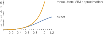
True solution and VIM approximations with N = 3 terms.
So we see that the linear function as the initial approximation does not work. Instead, we use its complementary function \( T_0 (x) = A\,\cos x + B\,\sin x . \) Then
\[
T_{1} (x) = A\,\cos x + B\,\sin x + \int_0^x \sin \left( s-x \right) \left\{ T''_0 (s) + T_0 (s) + 2s \right\} {\text d}s = A\,\cos x + \left( B+2 \right) \sin x -2x .
\]
By imposing the boundary conditions, we get A = 4 and \( B= 7\,\csc 2 - 4\,\cot 2 -2 . \) So
Now we consider the homogeneous equation corresponding to the given driven equation \( \ddot{y} + \omega^2 y =0 \) subject to the given initial conditions; its solution, called the complementary function, can be chosen as the initial approximation
\[
y_{0} (t) = C_1 \cos \omega t + C_2 \sin \omega t = \cos \omega t - \frac{\sin \omega t}{\omega} ,
\]
where C1 and C2 are such constants to satisfy the given initial conditions, y(0) = 1 and y'(0) = -1. Then the iteration formula gives
\begin{eqnarray*}
y_1 (t) &=& y_0 (t) - \frac{1}{\omega} \int_0^t \sin \omega (s-t) \left[ A\,\sin \omega s + B\,\sin \omega s \right] {\text d}s
\\
&=& C_1 \cos \omega t + C_2 \sin \omega t - \frac{A}{2} \left[ t\,\cos \omega t - \frac{\sin \omega t}{\omega} \right] + \frac{B\,\omega}{\omega^2 -1} \left[ \cos \omega t - \cos t \right] ,
\end{eqnarray*}
which is the general solution of the given differential equation (harmonic oscillator).
However, is we apply restricted variations to the correction function, then its exact solution can be arrived at only by successive iterations. Considering the corresponding homogeneous differential equation \( \ddot{y} + \omega^2 y =0 , \) we rewrite the correction functional as follows:
Here \( \tilde{y}_n (s) \) is considered a restricted variation, then the stationary conditions (\( \delta\tilde{y}_n =0 \) ) of the above correction functional can be expressed as follows
\[
\begin{split}
\lambda '' (s) &=0 ,
\\
\left. \lambda (s) \right\vert_{s=t} &= 0,
\\
\left. 1 - \lambda ' (s) \right\vert_{s=t} &= 0 .
\end{split}
\]
Therefore, the Lagrange multiplier becomes \( \lambda = s-t . \) This leads to the following iteration formula
Inan Ates and Ahmet Yildirim, "Comparison between variational iteration method and homotopy perturbation method for linear and nonlinear partial differential equations with the nonhomogeneous initial conditions," Numerical Methods for Partial Differential Equations, 2010, Vol 26, Issue 6, pp. 1581--1593, doi: https://doi.org/10.1002/num.20511
Ganji DD, Sadighi A (2006) Application of He’s methods to
nonlinear coupled systems of reactions. Int J Nonlinear Sci
Numer Simul 7(4):411–418
Ganji DD, Jannatabadi M, Mohseni E (2006) Application of He’s
variational iteration method to nonlinear Jaulent–Miodek equa-
tions and comparing it with ADM. Journal of Applied Mathematics and Computing, 207:35–45
Ganji DD, Tari H, Babazadeh H (2007) The application of He’s
variational iteration method to nonlinear equations arising in heat
transfer. Physics Letters A, Vol. 363, No. , pp. 213--217
Ganji DD, Tari H, Jooybari MB (2007) Variational iteration
method and homotopy perturbation method for evolution equations. Comput Math Appl 54:1018–1027
Ji-Huan He, "Variational iteration method---a kind of non-linear analytical technique: some examples," International Journal of Non-Linear Mechanics, 1999, Vol 34, 699--708.
Ji-Huan He, "Variational iteration method for autonomous ordinary differential systems," Applied Mathematics and Computation, 2000, Vol. 114, 115--123.
Ji-Huan He, Variational iteration method — Some recent resultsand new interpretations, Journal of Computational and Applied Mathematics, 2007, Vol. 207, pp. 3--17.
Rafei M, Daniali H, Ganji D,D., Variational iteration
method for solving the epidemic model and the prey and predator
problem, Applied Mathematics and Computation, 2007, Vol. 186, No. 2,
pp. 1701--1709.
S. S. Samaee, O. Yazdanpanah, and D. D. Ganji, "New approaches to identification of the Lagrange multiplier in the variational iteration method," Journal of the Brazilian Society of
Mechanical Sciences and Engineering, 2914, doi: 0.1007/s40430-014-0214-3
Tari H, Ganji D.D., Rostamian M. (2007) Approximate solution of
K (2, 2), KdV and modified KdV equations by variational itera-
tion method, homotopy perturbation method and homotopy ana-
lysis method. Int J Nonlinear Sci Numer Simul 8:203–210
Tatari M, Dehghan M (2007), "He’s variational iteration method
for computing a control parameter in a semi-linear inverse
parabolic equation," Chaos Solitons Fractals, 33(2):671--677.
A.-M. Wazwaz (2006), "A study on linear and nonlinear Schrodinger
equations by the variational iteration method," Chaos Solitons
Fractals, doi: 10.1016/j.chaos.10.009
A.-M. Wazwaz (2007), "The variational iteration method for solving
tow forms of Blasius equation on a half-infinite domain," Applied
Mathemathics and Computation, 2007, Vol. 188, Issue 1, pp. 485--491.
A.-M. Wazwaz (2007), The variational iteration method for the
exact solution of Laplace equation, Physics Letters A, Vol. 363, No 4, pp. 260--262, doi: 10.1016/j.physleta.2006.11.014
A.-M. Wazwaz (2001) The numerical solution of fifth-order
boundary value problems by the decomposition method. Journal of Applied Mathematics and Computing, 136:259–270
Wazwaz AM (2007) The variational iteration method for solving
a system of PDES. Comput Math Appl 54:895–902
Wu, B. S., C. W. Lim, and L. H. He, “A new methodfor approximate analytical solutions to nonlinear oscillations ofnonnatural systems,”Nonlinear Dynamics, Vol. 32, 1–13, 2003.
Return to Mathematica page
Return to the main page (APMA0330)
Return to the Part 1 (Plotting)
Return to the Part 2 (First Order ODEs)
Return to the Part 3 (Numerical Methods)
Return to the Part 4 (Second and Higher Order ODEs)
Return to the Part 5 (Series and Recurrences)
Return to the Part 6 (Laplace Transform)
Return to the Part 7 (Boundary Value Problems)