Return to computing page for the second course APMA0340
Return to computing page for the fourth course APMA0360
Return to Mathematica tutorial for the first course APMA0330
Return to Mathematica tutorial for the second course APMA0340
Return to Mathematica tutorial for the fourth course APMA0360
Return to the main page for the course APMA0330
Return to the main page for the course APMA0340
Return to the main page for the course APMA0360
Return to Part I of the course APMA0330
Glossary
Implicit Plot
You can use a variety of different plot functions to make graphs. In this section, I will introduce you to contour plot. The contour plot command gives the contour diagram of a function similar to what are known as "level curves" on a topographical map .
PlotRange -> {{-2, 2}, {-4, 4}}, AspectRatio -> 1.5/2.1,
ContourStyle-> {Green , Thickness[0.005]},
FrameLabel -> {"x", "y"}, RotateLabel -> False] (* Thickness is .5% of the figure's length *)
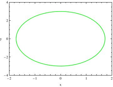
After I entered the ContourPlot command, use a variety of different commands to modify the graph and create a more aesthetically pleasing graph. When adding the details for plotting, do not close the ContourPlot command until all of the adjustments have been made.
PlotRange tells me the range that I want to plot. This is different from the x and y ranges before it because those numbers give the ranges that should be used to solve the given equation.
AspectRatio tells me the ratio between the height and the width of the graph. This describes how you want to scale the x-axis and y-axis to look in comparison with one another.
ContourStyle describes how you want the lines of the contour plot to look.
This command can also be used to change the color of the graph. If you do this, you need to add a second command with ContourStyle like I did above. For the Thickness command, this describes the percent thickness you want of the line, I have it set at .5% of the figure's length.
FrameLabel tells me what I want to be placed on the borders of the graph. For example, if I was graphing a Potential Energy Function, I could set the vertical frame to say U(x) and the horizontal frame to say x.
RotateLabel tells me whether or not I want to rotate the label that I designated using the FrameLabel Command.
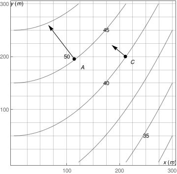
j=Graphics[{{PointSize[Large], Black, Point[{{115,195},{212,200}}]}, Inset["A", {130,180}], Inset["C", {225,190}], Inset["y(m)", {6,301}], Inset["x(m)", {295,0}], Inset["50", {100,200}], Inset["45", {175,250}], Inset["40", {175, 150}], Inset["35", {250,50}]}];
k= Graphics[Arrow[{{115,195}, {65,260}}]];
l= Graphics[Arrow[{{212,200}, {185,222}}]];
Show[i, j, k, l]
Another option:
j2 = Graphics[{{PointSize[Large], Black, Point[{{115, 195}, {212.132, 200}}]}, Inset["A", {130, 180}], Inset["C", {225, 190}], Inset["y(m)", {6, 301}], Inset["x(m)", {295, 0}], Inset["50", {100, 200}], Inset["45", {175, 250}], Inset["40", {175, 150}], Inset["35", {250, 50}]}];
k2 = Graphics[Arrow[{{115, 195}, {65, 260}}]];
l2 = Graphics[Arrow[{{212.132, 200}, {185, 222}}]];
Now it is right time to answer your question: Where did those points come from? Where did those arrows (vectors) come from?
sol1 = Solve[1/300 x^2 + 50 - y == 0, #] & /@ {x, y}
Below, the one on the right is on the 200 grid-line for the y axis. We add a grid-line to highlight the x value. We found the coordinates for the point which tells us where to put that grid-line from the equations above.
Because of LaGrange, Gram-Schmidt, Pythagoras, independence, orthogonality and a host of other important reasons, we often want to know the direction which is perpendicular to the tangent to the curve at a point. That is how we determine the vector, thus the other end of the arrow. The derivative of the function is the slope of a line tangent to the curve at a particular point. The perpendicular is when the dot product of the two vectors is zero...
% /. x -> 212.132
1/300 x^2 + 50 /. x -> 212.132
slope = %[[2, 2, 1]]
1.47421
{x0, y0} = {212.132, 200};
Caution: arrow along red line - coordinates for arrow point estimated by gridlines. Dot product may not be zero.
infLine2 = Graphics[{Thick, Red, InfiniteLine[{x0, y0}, {1, m}]}];
arrow = Graphics[{PointSize[Medium], Point[{{212.132, 200}}], Arrowheads[Medium], Thick, Arrow[{{212.132, 200}, {175, 225}}]}, PlotRange -> {{0, 200}, {0, 220}}];
Show[i2, j2, k2, infLine1, infLine2, arrow]
