Return to computing page for the second course APMA0340
Return to computing page for the fourth course APMA0360
Return to Mathematica tutorial for the first course APMA0330
Return to Mathematica tutorial for the second course APMA0340
Return to Mathematica tutorial for the fourth course APMA0360
Return to the main page for the course APMA0330
Return to the main page for the course APMA0340
Return to the main page for the course APMA0360
Return to Part III of the course APMA0330
Glossary
Preface
This chapter gives an introduction to numerical methods used in solving ordinary differential equations of first order. Its purpose is not to give a comprehensive treatment of this huge topic, but to acquaint the reader with the basic ideas and techniques used in numerical solutions of differential equations. It also tries to dissolve a myth that Mathematica is not suitable for numerical calculations with numerous examples where iteration is an essential part of algorithms.
Introduction to Numerical Methods
Ordinary differential equations are at the heart of our perception of the physical universe. Up to this point, we have discussed analytical methods for solving differential equations that involve finding an exact expression for the solution. It turns out that the majority of engineering and applied science problems cannot be solved by methods discussed so far or when they can be solved, the formulas become so complicated and cumbersome that it is very difficult to interpret them. For this reason development of numerical methods for their solutions is one of the oldest and most successful areas of numerical computations. A universal numerical method for solving differential equations does not exist. Every numerical solver can be flanked by some problem involving differential equation. Hence, it is important to understand the limitations of every numerical algorithm and apply it wisely. This chapter gives a friendly introduction to this topic and addresses basic ideas and techniques for their realizations. It cannot be considered as a part of the comprehensive numerical analysis course and the reader is advised to study other sources to pursue a deeper knowledge.
Actually, this chapter consists of two parts. The first six sections are devoted to solving nonlinear algebraic and transcendental equations that have many applications in all fields of engineering and it is one of the oldest and most basic problems in mathematics. They also serve as an introduction to the iterative methods that are widely used in all areas of numerical analysis and applied mathematics.
Mathematica has built-in functions Find Root, NSolve, Solve, Root that can solve the root-finding problems. However, programming the algorithms outlined below has great educational value. Besides, if you know what is under the hood, you can use it more efficiently or avoid misuse.
We present several algorithms that can be and some will be extended for solving differential equations numerically that constitute the second part of this chapter. Since solving nonlinear equations is one of the most important problems that has many applications in all fields of engineering and computer science, we start this chapter with an introduction to this topic. Note that we do not discuss specialized algorithms for finding roots of polynomials or solving systems of algebraic equations.
line = Graphics[{Black, Thick, Line[{{-1.1, -0.3}, {1.2, -0.3}}]}];
line2 = Graphics[{Black, Line[{{0, -1}, {1.2, -1}}]}];
w = Plot[{-0.3, -1.3}, {x, -1.13, 1.13}, Filling -> {1 -> {2}}, FillingStyle -> Cyan];
ar = Graphics[{Black, Arrowheads[{{-0.04}, {0.04}}], Arrow[{{1.25, -1}, {1.25, -0.3}}]}];
th = Graphics[{Black, Text[Style["h", 18], {1.35, -0.7}]}];
fill = Graphics[{LightBlue, Polygon[Table[{0.99 Cos[theta], 0.99 Sin[theta]}, {theta, Pi + 0.3, 2 Pi - 0.29, 0.05}]]}];
Show[line, line2, w, ar, th, circle, fill]
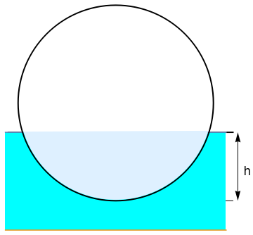
Applying Archimedes’ principle produces the following equation in term of h
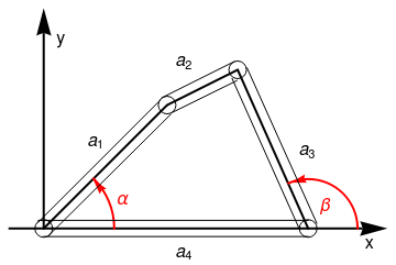
For any admissible value of the angle β, let us determine the value of the corresponding angle α between the rods a₄ and a₁. The vector identity holds:
Since the rod a₄ is always aligned horizontally, we can deduce the following relationship between β and α:
Let f be a real single-valued continuously differentiable function of a real variable. If f(α) = 0, then α is said to be a zero of f or, equivalently, a root of the equation f(x) = 0. In the first part of this chapter, we present several algorithms for finding roots of such equations iteratively:
Now we give a basic classification of iterative methods following J.F. Traub (1932--2015).
- If every step value xk+1 in an iteration method \( \displaystyle x_{k+1} = \phi \left( x_k \right) \) depends only on the one previous step xk, then the method is called a one-point iteration. Newton's method is an example of such a method. In differential equations, such an iteration method is called a one-step method.
- If the iteration function \( \displaystyle \phi \left( x_k , x_{k-1} , \ldots , x_{k-n+1} \right) \) depends on n previous steps, the iteration method is called a one-point method with memory. An example of an iteration function with memory is the well-known secant method. In differential equations, such a method is called a multistep method.
-
Another type of iteration functions is derived by using the expressions w1(xk), w2(xk), … , wm(xk), where xk is the common argument. The iteration function ϕ, defined as
\[ x_{k+1} = \phi \left( x_k , w_1 (x_k ), w_2 (x_k ) , \ldots , w_m (x_k ) \right) , \qquad k=0,1,2,\ldots , \]is called a multipoint iteration function without memory. The simplest examples are Steffensen's method and Traub--Steffensen's method. In differential equations, such a method is usually referred to as the Runge--Kutta method.
-
Assume that an iteration function ϕ has arguments zj, where each argument represents m + 1 quantities xj, w1(xj), w2(xj), … , wm(xj), m ≥ 1. The iteration function
\[ x_{k+1} = \phi \left( z_k , w_1 (z_k ), w_2 (z_k ) , \ldots , w_m (z_k ) \right) , \qquad k=0,1,2,\ldots , \]is called a multipoint iteration function with memory.
Intermediate Value Theorem: : Let f(x) be continuous on the finite closed interval [𝑎,b] and define
Theorem: : Suppose that f(x) ∈ C¹[𝑎,b] and \( \displaystyle f' (x) - p\,f(x) \ne 0 , \) where p is a real number, then the equation f(x) = 0 has at most one root in [𝑎,b].
Theorem: : If f(x) ∈ C¹[𝑎,b], f(𝑎) f(b) < 0 and \( \displaystyle f' (x) - p\,f(x) \ne 0 , \) where p is a real number, then the equation f(x) = 0 has a unique root in (𝑎,b).
It would be very nice if discrete models could provide calculated solutions to (ordinary and partial) differential equations exactly, but of course they do not. In fact in general they could not, even in principle, since the solution depends on an infinite amount of initial data. Instead, the best we can hope for is that the errors introduced by discretization will be small when those initial data are reasonably well-behaved.
In the second part of this chapter, we discuss some simple numerical methods applicable to first-order ordinary differential equations in normal form subject to the prescribed initial condition:
The finite difference approximations have a more complicated and intricate ""physics"" than the equations they are designed to simulate. In general, recurrences usually have more properties than their continuous analogous counterparts. However, this irony is no paradox; the finite differences are used not because the numbers they generate have simple properties, but because those numbers are simple to compute.
Numerical methods for the solution of ordinary differential equations may be put in two categories---numerical integration (e.g., predictor-corrector) methods and Runge--Kutta methods. The advantages of the latter are that they are self-starting and easy to program for digital computers but neither of these reasons is very compelling when library subroutines can be written to handle systems of ordinary differential equations. Thus, the greater accuracy and the error-estimating ability of predictor-corrector methods make them desirable for systems of any complexity. However, when predictor-corrector methods are used, Runge--Kutta methods still find application in starting the computation and in changing the interval of integration.
In this chapter, we discuss only discretization methods that have the common feature that they do not attempt to approximate the actual solution y = ϕ(x) over a continuous range of the independent variable. Instead, approximate values are sought only on a set of discrete points \( x_0 , x_1 , x_2 , \ldots . \) This set is usually called the grid or mesh. For simplicity, we assume that these mesh points are equidistant: \( x_n = a+ n\,h , \quad n=0,1,2,\ldots . \) The quantity h is then called the stepsize, stepwidth, or simply the step of the method. Generally speaking, a discrete variable method for solving a differential equation consists of an algorithm which, corresponding to each lattice point xn, furnishes a number yn which is to be regarded as an approximation to the true value \( \varphi (x_n ) \) of the actual solution at the point xn.
A complete analysis of a differential equation is almost impossible without utilizing computers and corresponding graphical presentations. We are not going to pursue a complete analysis of numerical methods, which usually requires:
- an understanding of computational tools;
- an understanding of the problem to be solved;
- construction of an algorithm that will solve the given mathematical problem.
In this chapter, we concentrate our attention on presenting some simple numerical algorithms for finding solutions of the initial value problems for first order differential equations in normal form:
Fundamental Inequality
We start with estimating elements of sequences.
Theorem: Suppose that elements of a sequence \( \left\{ \xi_n \right\} , \ n=0,1,2,\ldots , \) satisfy the inequalities of the form
Theorem: If A is a quantity of the form 1 + δ , then \( A = 1 + \delta < e^{\delta} \) and we have
We need to recall a very important definition.
Rudolf Otto Sigismund Lipschitz (1832--1903) was born in Königsberg, Germany (now Kaliningrad, Russia). He entered the University of Königsberg at the age of 15 and completed his studies at the University of Berlin, from which he was awarded a doctorate in 1853. By 1864 he was a full professor at the University of Bonn, where he remained the rest of his professional life.
Theorem (Fundamental Inequality): Let f(x,y) be a continuous function in the rectangle \( [a,b] \times [c,d] \) and satisfying the Lipschitz condition
Horner's Rule
As an illustration of an iteration procedure, we consider a very important problem that has a long history. We will discuss the marvelous problem of polynomial evaluation at any given point x = x0 that embraces different topics---synthetic division and Taylor polynomials (that is our future topic in chapter 5). Let us consider a polynomial in the variable x with real coefficients pn(x) of degree n
To check our conclusion, let us write a third-degree polynomial
Now we present a mesmerizing mathematical method called Horner's rule (or Horner's method, Horner's scheme, etc) for polynomial evaluation that requires fewer flops than any other algorithm. This method was described by the British mathematician William George Horner in 1819. However, it was published in 1803 by the Italian mathematician Paolo Ruffini (1765--1822); it can be traced back many hundreds of years to Chinese and Persian mathematicians (see historical notes in the article by A. Pathan and T. Collyer). Horner's rule is the most efficient method of evaluating a dense polynomial at a particular value, both in terms of the number of operations and even in terms of the number of registers. Thus, in any application where such evaluations are required, it is fast and efficient, and usually overlooked. Moreover, it also allows one to determine the values of function's derivatives at the same point recursively.
We can rewrite the same polynomial pn(x) in nested form by factoring out each power of x as far as it will go to obtain
Instead of utilizing the nested form for polynomial evaluation, we employ Ruffini's idea and exploit the polynomial remainder theorem that states that any polynomial f(x) of degree n can be represented as
| Algorithm | Ruffini's rule for the derivative of the polynomial |
|
The nested form of a polynomial contains the basic operation involving addition and multiplication:
𝑎 + x*( ). We saw the same operation previously when one polynomial is divided into another one.
As we know from precalculus, the quotient polynomial is obtained by Synthetic Division. Although Mathematica has a dedicated command: HornerForm, we implement Synthetic Division directly.
b[n] = l[[n]];
For[k = n - 1, 1 <= k, k--, b[k] = x*b[k + 1] + l[[k]]];
rem = b[1]; Print["remainder = ", rem] ;
B = Table[b[k], {k, 2, n}]]
In the code above, l is the list of coefficients written in increasing order:
rem, and the array B = [ q1 q2 … qn = 𝑎n ] that contains the list of coefficients of the quotient polynomial. Since this polynomial is one degree less than the given one, pn(x), we will denote by \( p_{n-1}(x) = a_n x^{n-1} + q_{n-1} x^{n-2} + \cdots + q_2 x + q_1 \) the quotient polynomial. Synthetic division is usually organized in the table.
| Coefficients: | 𝑎n | 𝑎n-1 | 𝑎n-2 | … | 𝑎1 | 𝑎0 | ||||||
|---|---|---|---|---|---|---|---|---|---|---|---|---|
| x0 | ↡ | x0*𝑎n | x0*qn-1 = x0(x0*𝑎n + 𝑎n-1) | … | x0*q2 | x0*q1 | ||||||
| Quotient: | 𝑎n | qn-1 = x0*𝑎n + 𝑎n-1 | qn-2 = x0(x0*𝑎n + 𝑎n-1) + 𝑎n-2 | … | q1 = x0*q2 + 𝑎1 | Remainder: x0*q1 + 𝑎0 |
Conclusions
Let us summarize what we achieved with synthetic division. With 2n flops (n additions and n multiplications), we determine the value of a polynomial with real coefficients of degree n
Example: We consider an example of polynomial evaluation at a point and its derivative using Horner's rule. Let
| Coefficients: | 2 | -3 | 0 | 5 | -7 | 9 | ||||||
|---|---|---|---|---|---|---|---|---|---|---|---|---|
| x0 = 3 | ↡ | 3*2 = 6 | 3*3 = 9 | 3*9 = 27 | 32*3 = 96 | 89*3 = 267 | ||||||
| Quotient: | 2 | 3*2 - 3 = 3 | 9+0 = 9 | 3*9 + 5 = 32 | 3*32 - 7 = 89 | Remainder = 276 |
We check with Mathematica
{89, 32, 9, 3, 2}
| Coefficients: | 2 | 3 | 9 | 32 | 89 | |||||
|---|---|---|---|---|---|---|---|---|---|---|
| x0 = 3 | ↡ | 3*2 = 6 | 3*9 = 27 | 3*36 = 108 | 3*140 = 420 | |||||
| Quotient: | 2 | 3*2 + 3 = 9 | 27 + 9 = 36 | 3*36 + 32 = 140 | Remainder = 509 |
{140, 36, 9, 2}
| Coefficients: | 2 | 9 | 36 | 140 | ||||
|---|---|---|---|---|---|---|---|---|
| x0 = 3 | ↡ | 3*2 = 6 | 3*15 = 45 | 3*81 = 243 | ||||
| Quotient: | 2 | 3*2 + 9 = 15 | 45 + 36 = 81 | Remainder = 383 |
{81, 15, 2}
| Coefficients: | 2 | 15 | 81 | |||
|---|---|---|---|---|---|---|
| x0 = 3 | ↡ | 3*2 = 6 | 3*21 = 63 | |||
| Quotient: | 2 | 3*2 + 15 = 21 | Remainder = 144 |
{21, 2}
| Coefficients: | 2 | 21 | ||
|---|---|---|---|---|
| x0 = 3 | ↡ | 3*2 = 6 | ||
| Quotient: | 2 | Remainder = 27 |
{2}
Horner's rule for polynomial evaluation

% the polynomial coefficients are stored in the array a(j), j=0,1,..,n

% px = value of polynomial upon completion of the code


px = a(n)

for k = n-1 downto 0

	px = a(k) + px*x

endfor
A similar algorithm for evaluating the derivative of a polynomial:
Horner's rule for polynomial derivative evaluation

% the polynomial coefficients are stored in the array a(j), j=0,1,..,n

% dp = value of derivative upon completion of the code


dp = n*a(n)

for k = n-1 downto 1

	dp = k*a(k) + dp*x

endfor
Horner's rule
was invented by
William George Horner (1786--1837) who was born in Bristol, England, and spent much of his life as a schoolmaster in
Bristol and, after 1809, in Bath. His paper on solving algebraic equations, which contains the algorithm we know as
Horner's rule, was published in 1819, although the Italian mathematician Paolo Ruffini (1765--1822) had previously
published a very similar idea.
There is a more efficient algorithm for polynomial evaluation:
A more efficient implementation of Horner's rule for polynomial evaluation

% the polynomial coefficients are stored in the array a(j), j=0,1,..,n

% b(n) = value of polynomial upon completion of the code


b(0) = a(n)

for k = 1 to n

	b(k) = x*b(k-1) + a(n-k)

endfor


% c(n-1) = value of derivative upon completion of the code


c(0) = b(0)

for k = 1 to n-1

	c(k) = x*c(k-1) + b(k)

endfor
- Bradie, B.A., Friendly Introduction to Numerical Analysis, Pearson Education,2007
- Burden, R.L. and Faires, J.D., Numerical Analysis, Cengage Learning, 10 edition, 2015.
- Chapra, S.C. and Canale, R.P., Numerical Methods, Online, The Hong Kong University of Science and Technology. 2012.
- Chasnov, J.R,, Numerical Methods, McGraw Hill,2009.
- Gerald C.F. and Wheatley, P.O., Applied Numerical Analysis, Pearson Education, 7th edition, 2003.
- Hauser, John R., Numerical Methods for Nonlinear Engineering Models, ISBN 978-1-4020-9920-5, 2009, Springer Netherlands, doi: 10.1007/978-1-4020-9920-5
- Ostrowski, A.M., Solutions of Equations and Systems of Equations, Academic Press, New York, 1960.
- Pathan A. and Collyer, T., The Wonder of Horner's Method, The Mathematical Gazette, Vol. 87, No. 509 (Jul., 2003), pp. 230-242
- Petković, M.S., Neta, B., Petković, L.D., Džunić, J., Multipoint Methods for Solving Nonlinear Equations, Elsevier, Amsterdam, 2013.
- Traub, J.F., Iterative Methods for Solution of Equations, Prentice-Hall, Englewood Cliffs, NJ, 1964.
- Wu, X., Wu, H.W., On a class of quadratic convergence iteration formulae without derivatives, Applied Mathematics & Computations, 2000, Vol. 10, Issue 7, pp. 381--389.
Return to Mathematica page
Return to the main page (APMA0330)
Return to the Part 1 (Plotting)
Return to the Part 2 (First Order ODEs)
Return to the Part 3 (Numerical Methods)
Return to the Part 4 (Second and Higher Order ODEs)
Return to the Part 5 (Series and Recurrences)
Return to the Part 6 (Laplace Transform)
Return to the Part 7 (Boundary Value Problems)