Preface
This section gives soem examples of plotting cycloids because they appear as solutions of some differential equations.
Return to computing page for the second course APMA0340
Return to computing page for the fourth course APMA0340
Return to Mathematica tutorial for the first course APMA0330
Return to Mathematica tutorial for the second course APMA0340
Return to Mathematica tutorial for the fourth course APMA0340
Return to the main page for the course APMA0330
Return to the main page for the course APMA0340
Return to the main page for the course APMA0360
Return to Part V of the course APMA0330
Glossary
Cycloids
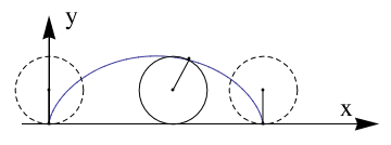
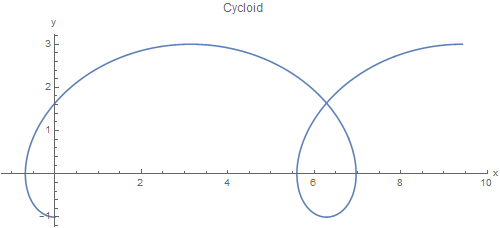
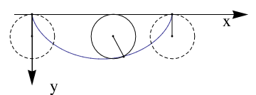
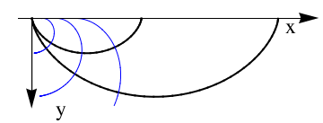
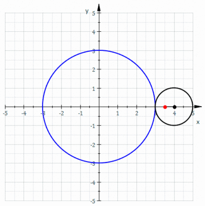
A cycloid is the curve traced by a point on the rim of a circular wheele, of radius 𝑎 rolling along a straight line. It was studied and named by Galileo in 1599. However, mathematical historian Paul Tannery cited the Syrian philosopher Iamblichus as evidence that the curve was likely known in antiquity. The history of cycloid was prepared by Tom Roidt. Its curve can be generalized by choosing a point not on the rim, but at any distance b from the center on a fixed radius. Alternatively, if we assume that the circle is turning at a constant rate, the parameter t could also be regarded as measuring the elapsed time since the circle began rolling. We will call the radius of our circle "𝑎." A graph of the cycloid curve and its generating circle, is presented beow. If b=𝑎, we get a usual cycloid.
Graphics[Join[{Arrowheads[a]},
Arrow[{{0, 0}, #}] & /@ {{x, 0}, {0, y}}, {Text[
Style["x", FontSize -> Scaled[f]], {0.9*x, .15*y}],
Text[Style["y", FontSize -> Scaled[f]], {0.07 x, 1*y}]}]]
data1 = Table[{t, cycloid[1, t][[1]], cycloid[1, t][[2]]}, {t, 0, 2 \[Pi], 0.01}];
Show[ListLinePlot[{#2, #3} & @@@ data1,
PlotRange -> {{-\[Pi]/4, 3 \[Pi]}, {0, 3}},
AspectRatio -> Automatic, Ticks -> {None, None}, Frame -> False,
PlotRange -> All, PlotRangeClipping -> False,
ImagePadding -> {{20, 20}, {20, 20}}], axes[9.7, 3.2, .07, .07],
Graphics[{{Dashed, Circle[{0, 1}, 1]}, Point[{\[Pi] + .5, 1}],
Point[{4.123, 1.9}], Circle[{\[Pi] + .5, 1}, 1],
Line[{{0, 0}, {0, 1}}], Point[{0, 0}], Point[{\[Pi]*2, 1}],
Point[{\[Pi]*2, 0}],
Point[{0, 1}], {Dashed, Circle[{\[Pi]*2, 1}, 1]},
Line[{{\[Pi]*2, 0}, {\[Pi]*2, 1}}],
Line[{{\[Pi] + .5, 1}, {4.123, 1.9}}]}]]
Another version:
|
Clear[f, g, theta];
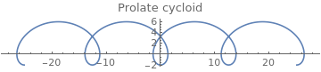
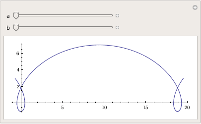
f[theta_] = 2 theta - 4 Sin[theta]; g[theta_] = 2 - 4 Cos[theta]; ParametricPlot[{f[theta], g[theta]}, {theta, -4*Pi, 4*Pi}, PlotLabel ->"Prolate cycloid"] |
Now we plot cycloid downward:
|
Graphics[Join[{Arrowheads[a]},
Arrow[{{0, 0}, #}] & /@ {{x, 0}, {0, y}}, {Text[ Style["x", FontSize -> Scaled[f]], {0.9*x, .08*y}], Text[Style["y", FontSize -> Scaled[f]], {0.1 x, 1*y}]}]] data1 = Table[{t, cycloid[1, 1][t][[1]], cycloid[1, 1][t][[2]]}, {t, 0, 2 \[Pi], 0.01}]; Show[ListLinePlot[{#2, -#3} & @@@ data1, PlotRange -> {{-\[Pi]/4, 3 \[Pi]}, {-3, 0}}, AspectRatio -> Automatic, Ticks -> {None, None}, Frame -> False, PlotRange -> All, PlotRangeClipping -> False, ImagePadding -> {{20, 20}, {20, 20}}], axes[9.7, -3.2, .07, .07], Graphics[{{Dashed, Circle[{0, -1}, 1]}, Point[{\[Pi] + .5, -1}], Point[{4.123, -1.9}], Circle[{\[Pi] + .5, -1}, 1], Line[{{0, 0}, {0, -1}}], Point[{0, 0}], Point[{\[Pi]*2, -1}], Point[{\[Pi]*2, 0}], Point[{0, -1}], {Dashed, Circle[{\[Pi]*2, -1}, 1]}, Line[{{\[Pi]*2, 0}, {\[Pi]*2, -1}}], Line[{{\[Pi] + .5, -1}, {4.123, -1.9}}]}] |
Graphics[Join[{Arrowheads[a]},
Arrow[{{0, 0}, #}] & /@ {{x, 0}, {0, y}}, {Text[
Style["x", FontSize -> Scaled[f]], {0.9*x, .08*y}],
Text[Style["y", FontSize -> Scaled[f]], {0.1 x, 1*y}]}]]
data1 = Table[{\[Tau], Cycloid[1, \[Tau]][[1]],
Cycloid[1, \[Tau]][[2]]}, {\[Tau], 0, 2 \[Pi], 0.01}];
data2 = Table[{\[Tau], Cycloid[1.5, \[Tau]][[1]],
Cycloid[1.5, \[Tau]][[2]]}, {\[Tau], 0, 3.14^2 - 0.6, 0.01}];
data1a = Table[{\[Rho], Cycloid[\[Rho], 2][[1]],
Cycloid[\[Rho], 2][[2]]}, {\[Rho], .3, 10, .01}];
data2a = Table[{\[Rho], Cycloid[\[Rho], 3][[1]],
Cycloid[\[Rho], 3][[2]]}, {\[Rho], .5, 10, .01}];
data3a = Table[{\[Rho], Cycloid[\[Rho], 4][[1]],
Cycloid[\[Rho], 4][[2]]}, {\[Rho], .65, 10, .01}];
Show[ListLinePlot[{#2, -#3} & @@@ data1, AspectRatio -> Automatic,
PlotRange -> {{-\[Pi]/4, 5*\[Pi]}, {-5, 0}},
PlotStyle -> {Black, Thick}, Ticks -> {None, None}, Frame -> False,
PlotRange -> All, PlotRangeClipping -> False,
ImagePadding -> {{20, 20}, {20, 20}}],
ListLinePlot[{#2, -#3} & @@@ data2, PlotStyle -> {Black, Thick},
PlotRange -> {{-\[Pi]/4, 2*\[Pi] + \[Pi]/4}, {-5, 0}},
Ticks -> {None, None}, Frame -> False, PlotRange -> All,
PlotRangeClipping -> False, ImagePadding -> {{20, 20}, {20, 20}}],
ListLinePlot[{#2, -#3} & @@@ data1a,
PlotRange -> {{-\[Pi]/4, 2*\[Pi] + \[Pi]/4}, {-5, 0}},
Ticks -> {None, None}, Frame -> False, PlotRange -> All,
PlotStyle -> {Blue}, PlotRangeClipping -> False,
ImagePadding -> {{20, 20}, {20, 20}}],
ListLinePlot[{#2, -#3} & @@@ data2a,
PlotRange -> {{-\[Pi]/4, 2*\[Pi] + \[Pi]/4}, {-5, 0}},
Ticks -> {None, None}, Frame -> False, PlotRange -> All,
PlotStyle -> {Blue}, PlotRangeClipping -> False,
ImagePadding -> {{20, 20}, {20, 20}}],
ListLinePlot[{#2, -#3} & @@@ data3a,
PlotRange -> {{-\[Pi]/4, 2*\[Pi] + \[Pi]/4}, {-5, 0}},
Ticks -> {None, None}, Frame -> False, PlotStyle -> {Blue},
PlotRange -> All, PlotRangeClipping -> False,
ImagePadding -> {{20, 20}, {20, 20}}], axes[16.5, -5.2, .07, .07]]
Trochoid

Manipulate[
ParametricPlot[
trochoid[a, b][t] // Evaluate, {t, -\[Pi]/2, 5*\[Pi]/2}], {a, 1, 5}, {b, 1, 5}]
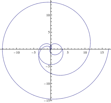
PolarPlot[Cycloid[1.5,theta],{theta, 0, 4*Pi}]
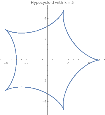
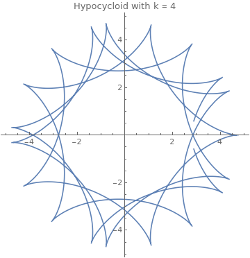
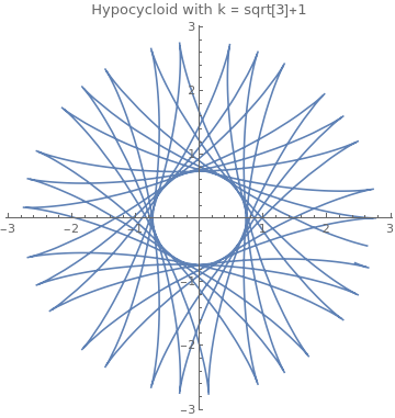
Hypocycloid
|
ParametricPlot[{4*Cos[theta] + Cos[4*theta],
4*Sin[theta] - Sin[4*theta]}, {theta, -4*Pi, 8*Pi},
PlotLabel -> "Hypocycloid"]
|
If k is a rational number, say k = p/q expressed in simplest terms, then the curve has p cusps.
|
ParametricPlot[{3.7*Cos[theta] + Cos[3.7*theta],
3.7*Sin[theta] - Sin[3.7*theta]}, {theta, -4*Pi, 4*Pi},
PlotLabel -> "Hypocycloid with k = 4.7"]
|
If k is an irrational number, then the curve never closes, and fills the space between the larger circle and a circle of radius R − 2r.
|
ParametricPlot[{Sqrt[3]*Cos[theta] + Cos[Sqrt[3]*theta],
Sqrt[3]*Sin[theta] - Sin[Sqrt[3]*theta]}, {theta, -8*Pi, 14*Pi},
PlotLabel -> "Hypocycloid with k = 4.7"]
|
Epitrochoid
Return to Mathematica page
Return to the main page (APMA0330)
Return to the Part 1 (Plotting)
Return to the Part 2 (First Order ODEs)
Return to the Part 3 (Numerical Methods)
Return to the Part 4 (Second and Higher Order ODEs)
Return to the Part 5 (Series and Recurrences)
Return to the Part 6 (Laplace Transform)
Return to the Part 7 (Boundary Value Problems)