Since the Gibbs phenomenon predicts overshoots and undershoots at the
points of discontinuity that are proportional to the size of the jump, this
section shows how this coefficient of proportionality, called Wilbraham's
constant, can be numerically determined. Its derivation comes up in two
cases: either when the point of discontinuity is within the interval
or when it is at the end points of the main interval.
The idea behind its derivation is very similar in both cases. First, we
consider the truncated finite Fourier series of the function responsible for the jump
of discontinuity, differentiate it, and then determine critical points where the
derivative is zero. Next substitution of these critical points into the finite
Fourier series yields the
finite Riemann
sum for the sine integral \( \mbox{Si}(x)
= \int_0^x \frac{\sin t}{t}\,{\text d}t \) in both cases.
Taking the limit gives the numerical value of the undershoot/overshoot.
Return to computing page for the first course APMA0330
Return to computing page for the second course APMA0340
Return to Mathematica tutorial for the first course APMA0330
Return to Mathematica tutorial for the second course APMA0340
Return to the main page for the first course APMA0330
Return to the main page for the second course APMA0340
Return to Part V of the course APMA0340
Introduction to Linear Algebra with Mathematica
A periodic function of period 2ℓ from the Dirichlet theorem (that guarantees the pointwise convergence of the Fourier series to the given function) has on the interval
[-ℓ,ℓ] a discrete number
of discontinuities
of finite jumps and the given interval [-ℓ,ℓ] can be divided
into a finite number of subinterval so that on each of them the function
is either monotonically increasing or decreasing. Such functions are
called functions of finite (or bounded) variations. Discontinuities of such functions can occur in two cases: either within the interval or at the end points when the Fourier series periodically extends the given function. Since the Gibbs phenomenon can be observed only at the points of discontinuity, it is sufficient to consider only two cases when the function has a jump inside the interval (-ℓ,ℓ) or when the values of the function at end points are distinct.
Discontinuity in the middle of the interval
Without any loss of generality, we can assume that the function under
consideration has only one
finite jump within the interval (-ℓ,ℓ) because any function of finite
variation can be represented as a finite sum of such functions. Let
x0 denote an x-value where such a jump occurs; it is
at most a matter of translation of coordinate system and perhaps a reflection
to assume that x0 = 0.
Let us assume that the left and right limits of f(x) at the
point of discontinuity are \( -a = f(0-0) =
\lim_{\varepsilon \to 0} \,f(-\varepsilon ) , \quad b = f(0+0) =
\lim_{\varepsilon \to 0} \,f(\varepsilon )
\) (where limits were calculated for positive ε).
The derivation of Wilbraham's constant for a function having only one
finite jump of value a+b at the origin can be broken down into the
following steps.
Construct a step function that has exactly the same jump of discontinuity as
the given function at the origin.
Subtract the step function found in the previous step from the given function
to obtain the continuous function that we denote
by g(x).
Expand the step function into the Fourier series. We denote by
\( \displaystyle S_N (x) = \frac{a_0}{2} +
\sum_{k=1}^N a_k \cos \frac{k\pi x}{\ell} + b_k \sin \frac{k\pi
x}{\ell} \) its partial finite Fourier
sum with N+1 terms. Since
g(x) is a periodic continuous function on the interval (-ℓ,ℓ), its Fourier
series does not exhibit the Gibbs phenomenon.
Determine critical points of the finite Fourier series
SN(x) by equating its derivative to zero and solving
the corresponding transcendent equation.
Identify the critical point that is closest to the origin (point of
discontinuity) and where the function SN(x)
attains maximum or minimum.
Evaluate the finite Fourier sum SN(x) at the above critical
point.
Show that this finite Fourier series at the critical point is actually a
Riemann sum
for sine integral \( \mbox{Si}(x)
= \int_0^x \frac{\sin t}{t}\,{\text d}t \) at point x
= π.
Find the limit when \( N\mapsto \infty \) to
determine the numerical value of Wilbraham's
constant.
We can observe such a function through the following step function:
\[
s(x) = \begin{cases}
b , & \ \mbox{ for } \ x > 0 , \\
(b-a)/2 , & \ \mbox{ for } \ x=0 , \\
-a , & \ \mbox{ for } \ x < 0 .
\end{cases}
\]
This step function has jump of a+b at the origin and it can be represented as a linear combination of the Heaviside functions:
because the sum of two Heaviside functions is identically 1:
\[
H(t) + H(-t) = 1 .
\]
Since the Heaviside function
\[
H(t) = \begin{cases}
1, & \ \mbox{ for } \ t > 0 , \\
1/2, & \ \mbox{ for } \ t =0 , \\
0, & \ \mbox{ for } \ t < 0 ,
\end{cases}
\]
has jump of discontinuity of unit length at the origin, the difference of them,
s(x) = H(x) - H(-x), will have a symmetric jump of value
2. Although an arbitrary discontinuous function may have asymmetric jump of
value (a+b) at the origin, we can always extract from it the
function \( \frac{a+b}{2} \left[ H(t) - H(-t) \right] +
\frac{b-a}{2} \) so the rest will be a continuous function. Therefore,
it is sufficient to consider the Fourier series for the difference of two
Heaviside functions (with symmetric jump), which we denote by S:
\[
S(t) \equiv H(t) - H(-t) =
\frac{4}{\pi}\,\sum_{n\ge 1} \frac{\sin \frac{(2n-1)\pi t}{\ell}}{2n-1}
= \begin{cases}
1, & \ \mbox{ for } \ t > 0 , \\
0, & \ \mbox{ for } \ t =0 , \\
-1, & \ \mbox{ for } \ t < 0 .
\end{cases}
\]
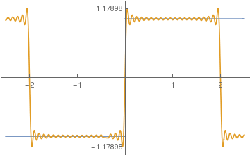
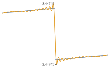
Then we plot the step function \( S(t) = H(t) - H(-t)
\) along with its 20-term Fourier approximation for ℓ = 2:
So at these points the partial Fourier sums attain alternating maximum and
minimum.
The first closest point to the origin is t0 = ℓ/2/N. Hence at this point, the partial Fourier sum becomes
where Si(x) = \( \int_0^x \frac{\sin
t}{t}\,{\text d}t \) is the sine integral (special
function).
N[SinIntegral[Pi]/Pi, 20]
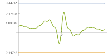
To confirm that the maximum oscillation occurs at the point above, we
can observe another critical point. At this point, the partial sum
will approach a smaller value
than 2w. In addition, the second ripple will be about 1.59, which is seen from
the above picture.
Discontinuity at the end points
Suppose that the given function f(x) on the interval
[-ℓ, ℓ] has not equal values at the end points; suppose that the
values of the function at end poinst are f(-ℓ) = -a and
f(ℓ) = b, where a ≠ b.
Identify a linear function l(x) that has the same values at
the end points as the given function.
Add the linear function found in the previous step to the given function
to obtain the continuous function that we denote by φ(x)
Expand the linear function into the Fourier series. We denote by
SN(x) its partial finite Fourier
sum with N terms. Since
φ(x) is continuous at the end points of the interval (-ℓ,ℓ), its Fourier
series does not exhibit the Gibbs phenomenon.
Determine critical points of the finite Fourier series
SN(x) by equating its derivative to zero and solving
the corresponding transcendent equation.
Identify the critical point that is closest to the end point and where the
function SN(x)
attains maximum or minimum.
Evaluate the finite sum SN(x) at the above critical
point.
Show that this finite Fourier series at the critical point is actually a
Riemann sum for sine integral.
Find the limit when \( N\mapsto \infty \) to
determine the numerical value of Wilbraham's constant.
We can observe such a fuction if we subtract from
f(x) the linear function
\[
l(x) = \frac{b+a}{2}\, x + \frac{b-a}{2} ,
\]
the result will be a continuous function at end points. Therefore, we can
consider only a linear function
Since the cosine is positive on the given interval, cosθ > 0 for
-π/2 < θ < π/2, we need to equate the other two functions to zero
and obtain two sequences of zeroes:
Hence, we conclude that overshoot and undershoot at end points will
be again equal to \( \frac{a+b}{2}\, w = \frac{a+b}{2}\,
0.0894899\ldots . \)
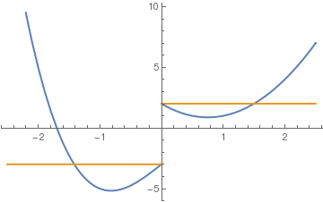
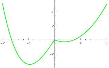
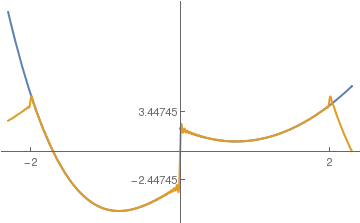
Let us consider the following piecewise continuous function on the interval
[-2,2]:
\[
f(x) =
\begin{cases}
2\,x^2 - 3\,x +2, & \ \mbox{ for } \ x > 0 , \\
1/2, & \ \mbox{ for } \ x =0 , \\
-2\, x^3 + 4\,x -3, & \ \mbox{ for } \ x < 0 .
\end{cases}
\]
This function has one internal point x = 0 of finite jump
of 5 units and discontinuities at end points because f(-2) = 5 and
f(2) = 4. To eliminate discontinuity at the origin, we subtract from
the given function the piecewise step function
\[
s(x) =
\begin{cases}
2, & \ \mbox{ for } \ x > 0 , \\
-1/2, & \ \mbox{ for } \ x =0 , \\
-3, & \ \mbox{ for } \ x < 0 .
\end{cases}
\]
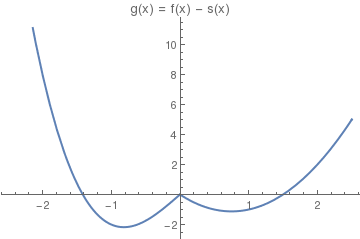
Then the resulting function \( g(x) = f(x) - s(x) \)
will be continuous at the origin.
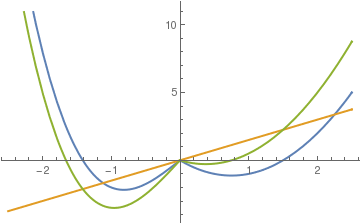
However, the function g(x), when extended periodically from the
interval [-2,2], will have discontinuities at these end points. Therefore, we
need to add to it the linear function l(x) = 3x/2,
so that the sum φ(x) = g(x) +
l(x) will have the same values at the end points.
\[
\varphi (x) =
\begin{cases}
2\,x^2 + \frac{3}{2}\,x , & \ \mbox{ for } \ x > 0 , \\
0, & \ \mbox{ for } \ x =0 , \\
-2\, x^3 + \frac{11}{2}\,x , & \ \mbox{ for } \ x < 0 .
\end{cases}
\]
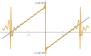
Now we expand the two functions, piecewise continuous function
f(x) and continuous function φ(x) into
Fourier series over the interval [-2,2].
Upon evaluating integrals on the interval [-2,2]
Fourier approximation with 100 terms of the given function.
■
Fay, T.H. and Kloppers, P.H., The Gibbs' phenomenon, International Journal of Mathematical Education in Science and Technology, 2001, Vol. 32, No. 1, pp. 73--89; doi:10.1080/00207390117151
Return to Mathematica page
Return to the main page (APMA0340)
Return to the Part 1 Matrix Algebra
Return to the Part 2 Linear Systems of Ordinary Differential Equations
Return to the Part 3 Non-linear Systems of Ordinary Differential Equations
Return to the Part 4 Numerical Methods
Return to the Part 5 Fourier Series
Return to the Part 6 Partial Differential Equations
Return to the Part 7 Special Functions