In many applications, a vector space under consideration is too large to provide an insight to the problem. It leads to looking at smaller subsets that are called subspaces as they inherit vector addition and scalar multiplication from the larger space. As a rule, subspaces occur in three cases: as a null space of a homogeneous equation, as a span of some vectors, or when an auxiliary condition is imposed on the elements of the large space. Three examples following the definition clarify theses cases.
A subset W of a vector space V is called a subspace of
V if W is itself a vector space under the addition and scalar
multiplication defined on V.
The linear span
(also called just span) of a set of vectors in a vector space is the
intersection of all linear subspaces which each contain every vector in that
set. Alternatively, the span of a set S of vectors may be defined as
the set of all finite linear combinations of elements of S.
The linear span of a set of vectors is therefore a vector space.
Example 2:
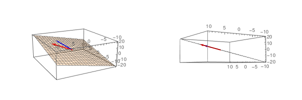
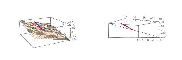
Let us consider the homogeneous differential equation
where ω is a positive number. Its general solution
\[
y(x) = C_1 \cos\omega x + C_2 \sin \omega x
\]
depends on two arbitrary constants. So the differential operator \( \displaystyle L\left[ \texttt{D} \right] = \texttt{D}^2 + \omega^2 , \) where \( \texttt{D} = {\text d}/{\text d}x , \) has a two-dimensional null-space that spans on two functions, cos(ωx) and sin(ωx).
Every vector space V has at least two subspaces: the whole space itself
V ⊆ V and the vector space consisting of the single element---the zero vector, {0} ⊆ V.
These subspaces are called the trivial subspaces. All other subspaces
(if any) are called proper subspaces. Perhaps the name "sub vector
space" would be better, but the only kind of spaces we consider are vector spaces, so "subspace" will do. Conversely, every vector space is a subspace of itself and possibly of other larger spaces.
In general, to show that a nonempty set W with two operations
(inner operation is usually called addition and outer operation of
multiplication by scalars) is a vector space one must verify the eight vector
space axioms. However, if W is a
subspace of a known vector space V, then certain axioms need not be
verified because they are "inherited" from V. For example,
commutative property needs not to be verified because it holds for all
vectors from V.
Theorem 1:
If W is a nonempty set of vectors from a vector space V, then
W is a subspace of V if and only if the following conditions
hold.
The zero vector of V is in W.
If u and v are vectors in W, then u + v is in W.
If k is a scalar and u is a vector in W, then ku is in W. ▣
So just three conditions, plus being a subset of a known vector space, gets us all eight postulates used to define of a vector space. Fabulous! This theorem can be paraphrased by saying that a subspace is “a nonempty subset (of a vector space) that is closed under vector addition and scalar multiplication."
Corollary 1:
Let V be an 𝔽-vector space (where 𝔽 is either ℝ or ℚ or ℂ) and let U be a nonempty subset of V. Then U is a subspace of V if and only if ku + v ∈ U whenever u, v ∈ U and k ∈ 𝔽.
If U is a subspace of V, then ku + v ∈ U whenever u, v ∈ U and k ∈ 𝔽 because a subspace is closed under scalar multiplication and vector addition.
Conversely, suppose that ku + v ∈ U whenever u, v ∈ U and k ∈ 𝔽. We must verify the properties:
Sums and scalar multiples of elements of U are in U (that is, U is closed under vector addition and scalar multiplication).
U contains the zero vector of V.
U contains an additive inverse for each of its elements.
Let u ∈ U. Then (−1)u is the additive inverse of u, so 0 = (−1)u + u ∈ U. This verifies part (b). Since (−1)u = (−1)u = ,b.0,/b., it follows that the additive inverse of u is in U. This verifies part (c). We have ku = ku + 0 ∈ U and u + v = 1u + v ∈ U. This verifies part (a).
Example 5:
The vector space ℝ² is not a subspace of ℝ³ because ℝ² is not even a subset of ℝ³. The vectors in ℝ² all have two coordinates, whereas the vectors in ℝ³ have three components.
On the other hand, the set (we use the ket notation |x> for column vector)
\[
V = \left\{ | {\bf x} > \, = \begin{pmatrix} a \\ 0 \\ b \end{pmatrix}\, : \, a \mbox{ and } b \mbox{ are real numbers} \right\}
\]
is a subset of ℝ³ that "looks" and "acts" like ℝ², although it is logically distinct from ℝ². We say in this case that the space V is isomorphic (see also section) to ℝ².
We check all three conditions of Corollary 1. Indeed, when 𝒶 = b = 0, we get a zero vector, so V. Using properties of real numbers, we get
because the nonhomogeneous vector (4, 0, 0) is doubled.
Another way to view it is that there is only one equation and two unknowns. The 2nd and 3rd rows are mere tautologies: x₂ + 0 + 0 = x₂ and x₃ = 0 + x₃ + 0 = x₃.
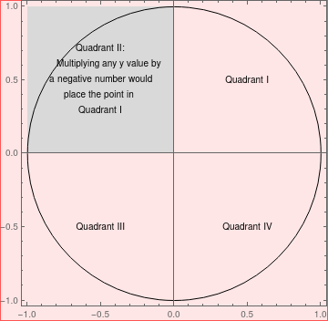
Example 8:
Let U be the set of all points (x, y) in ℝ² for which x ≤ 0 and y ≥ 0 (second quadrant). This set is not a subspace of ℝ² because it is not closed under scalar multiplication by a negative number.
Second quadrant
Graphics[{Style[RegionUnion[Rectangle[{-1, 0}]], LightGray], {Black,
Circle[{0, 0}, 1], Red,
Arrow[Circle[{0, 0}, .25, {2 \[Pi], \[Pi]/4}]]}},
Epilog -> {Text[
"Quadrant II:\n Multiplying any y value by\na negative \
number would\nplace the point in \nQuadrant I", {-.5, .5}],
Text["Quadrant I", {.5, .5}], Text["Quadrant III", {-.5, -.5}],
Text["Quadrant IV", {.5, -.5}]}, Axes -> True, Frame -> True
]
■
End of Example 8
Theorem 3:
Let W be a subspace of an n dimensional vector space V.
Then W is finite dimensional and dimW ≤ n, with
equality if and only if W = V.
If V = {0}, then dimU = 0 and there is nothing to prove;
so we may assume that V ≠ {0}. Let v1 ∈
V be nonzero. If span{v1} = U, then dimV
= 1. If span{v1} ≠ V, then there is a
v2 ∈ V such that the set {v1,
v2} is linearly independent. If span{v1,
v2} = V, then dimV = 2; otherwise, there exists
v3 ∈ V such that the set {v1,
v2, v3} is linearly independent. Repeat
until a linearly independent spanning list is obtained. Since no linearly
independent set of vectors in U contains more than n elements,
this process terminates in r ≤ n steps with a linearly
independent set of vectors v1, v2, ... ,
vr whose span is V. Thus, r = dimV
≤ n with equality only if v1,
v2, ... , vn is a basis for U.
Example 8: The set of monomials \( \left\{ 1, x, x^2 , \ldots , x^n \right\} \)
form a basis in the set ℘≤n of all polynomials of degree up to n. It has dimension n+1. It is a subspace of the vector space of all polynomials ℘. However, the set of polynomials of degree n is not a subspace of ℘≤n or ℘ because it is not closed under additions. For example, the sum of two polynomials
However, the set of all polynomials of even degree is a subset of the vector space ℘. For example, the set V of all polynomials of even degree up to two is a subset of ℘≤2, which dimension is 3. On other hand, V has dimension 2 because it is spanned on two monomials { 1, x² }.
■
End of Example 9
Fundamental Subspaces
Let A be an m × n matrix over either the field of real numbers ℝ or complex numbers ℂ. The space of all such matrices is denoted by ℳm,n(𝔽) or simply ℳm,n. Then A determines four important vector spaces known as the fundamental subspaces determined by A. They are column space 𝒞(A), the row space ℛ(A), the null space 𝒩(A), also called the kernel of matrix A denoted by ker(A), and cokernel of matrix A, denoted coker(A), which is the null space of adjoint matrix A*. In other words, the cokernel of matrix A includes all vectors such that
Two of these spaces (ℛ(A) and ker) are subspaces of 𝔽n and two of them (𝒞(A) and coker) are subspaces of 𝔽m. These subspaces will discussed in detail in further sections.
Theorem 4:
Suppose that A∈ℳm,n(𝔽) is an m×n matrix under field 𝔽 (either ℚ or ℝ or ℂ). Then its null space (also known as kernel) is a subspace of 𝔽n.
We will examine the two requirements of Theorem 1. First, we check that it is not empty. It is obviously true because the null space contains a zero vector.
Second, we check addition closure by taking two arbitrary vectors v and u from the null space. Since
Example 9:
Let us consider ℳm,n(ℝ), the set of all real m × n
matrices, and let \( {\bf M}_{i,j} \) denote the matrix whose only nonzero entry is a 1 in
the i-th row and j-th column. Then the set \( {\bf M}_{i,j} \ : \ 1 \le i \le m , \ 1 \le j \le n \)
is a basis for the set of all such real matrices. Its dimension is mn.
Let A ∈ ℳm,n(ℝ) and let U be a subspace of ℳm,n(ℝ). Then the set
is a subspace of ℳm,n(ℝ). Since 0 ∈ U, we have 0 = A0 ∈ U, which is therefore not empty. Moreover, kAX + AY = A(kX + Y) ∈ U for any scalar k and any X, Y ∈ U. Corollary 1 ensures that AU is a subspace of ℳm,n(ℝ). For example, we take U = ℳ3,3(ℝ) and
Theorem 5:
Suppose that A ∈ ℳm,n(𝔽) is an m×n matrix under field 𝔽 (either ℚ or ℝ or ℂ). Then its column space 𝒞(A) is subspace of 𝔽n.
A column space 𝒞(A) is spanned of columns of matrix A.
Then it consists of all possible linear combinations of the colon vectors. To prove closure under addition, let
which is a linear combination of column vectors, so it belongs to 𝒞(A). Similarly, it can be shown that this set is closed under scalar multiplication.
So span is a subspace of 𝔽n.