Today more than ever, electronics are an integral part of our everyday lives.
They contribute to every aspect of our way of life from lighting the space
around our work environments, to exploring uncharted territories. But behind
each and every electrical appliance or device, no matter what task it was
designed for, lies a vast system of electrical components that must function
as a whole. Each component (resistors, capacitors, inductors, etc.) has
specifications of their own, as does the final product that they are a part
of, so engineers must design their devices to meet not only their intended
purpose, but so that the individual components are within their tolerances.
Vital to this is the analysis of currents and voltages throughout the
electrical circuit. (Tiang, 2001)
Linear algebra is an essential tool when working with electric circuits. The
use of matrices is considered to be an integral concept utilized by electrical
engineers. Most of computer applications are based on linear algebra including
solutions of systems of linear equations.
Aside from the traditional approach of evaluating circuits by looking at the
left most and right most elements, there are many other choices when it comes
to solving electric circuit problems. Initially, an individual can begin
solving the circuit problem by looking at the output portion of the matter and
work back towards the input portion of the circuit. In other words, there are
multiple approaches to circuity problems, aside from a traditional approach of
evaluating the circuit from looking at the leftmost elements to the rightmost
elements.
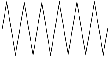
A resistor is a passive two-terminal electrical component that implements electrical resistance as a circuit element. In electronic circuits, resistors are used to reduce current flow, adjust signal levels, to divide voltages, bias active elements, and terminate transmission lines, among other uses.
The behavior of an ideal resistor is dictated by the relationship specified
by Ohm's law:
\[
V = R\,I ,
\]
where I is the current through the conductor in units of amperes, V is the voltage measured across the conductor in units of volts, and R is the resistance of the conductor in units of ohms.
The typical schematic diagram symbol for resistor is
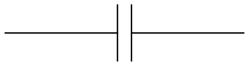
A capacitor is a passive two-terminal electrical component that stores potential energy in an electric field. The effect of a capacitor is known as capacitance. While some capacitance exists between any two electrical conductors in proximity in a circuit, a capacitor is a component designed to add capacitance to a circuit. The typical schematic diagram symbol for capacitor is
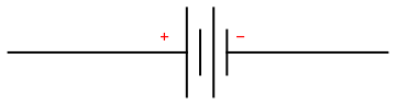
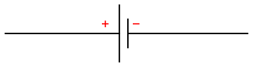
An electric battery is a device consisting of one or more electrochemical cells with external connections provided to power electrical devices such as flashlights, smartphones, and electric cars. When a battery is supplying electric power, its positive terminal is the cathode and its negative terminal is the anode. The terminal marked negative is the source of electrons that when connected to an external circuit will flow and deliver energy to an external device. The following symbol for a battery is used in a circuit diagram.
Example:
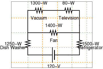
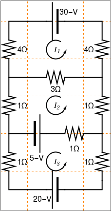
In Figure 1 below, we present a circuit diagram, representing a collection
of typical household appliances, connected (perhaps unsafely) to a single wall
outlet. The power that each appliance uses is listed in the figure, along with
the voltage provided by the outlet. The problem is to predict the amount of
current that is required to run all the appliances at once. This information
can be important, since if too much current is drawn from the outlet, a fuse
will fail and you will lose to power to all appliances.
In order to find the current passing through the outlet, we need to find the
current running through each appliance and the voltage at various places in
the circuit.
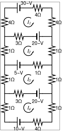
The first step in analyzing this circuit is to find the resistance of each
appliance. Using the information supplied by the manufacturer, the resistance
for each appliance can be determined. Figure 2 shows the resistance of each
appliance, and also the remaining unknown currents and voltages.
■
Developing linear equations from electric circuits is based on two Kirchhoff's
laws:
Kirchhoff's current law (KCL): at any node (junction) in an electrical circuit, the sum of currents flowing into that node is equal to the sum of currents flowing out of that node
Kirchhoff's voltage law (KVL): the sum of the emfs in any closed loop is equal to the sum of the potential drops in that loop.
The voltage drop (in volts) across resistor is approximately described by Ohm's law: V = R I, where
R is resistance (in ohms), I is current (this symbol was used by André-Marie Ampère, after whom the unit of electric current is named). There two things to remember:
when we travel around a loop of the circuit, the algebraic sum of the volts
has to be equal to zero;
always start at the battery.
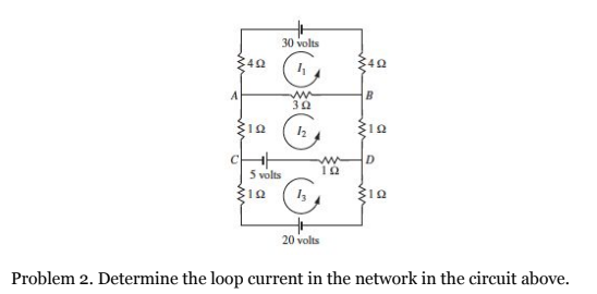
Example:
Consider a simple circuit with two resistors depictured in the figure.
Two loop circuit
Since the above circuit consists of two loops, we derive equations between
voltage v and current i for each loop. For the first circuit, we
use the following steps:
Starting from the battery our direction is going from the - to the + position, counter clockwise. Therefore,
we have a positive volt number: 12 v.
Traveling to the 2 Ω, we notice that the 2 Ω is being shared by
both circuits. Once again, we calculate by using the circuit that we are in
subtracted by the other circuit:
\[ _
12\,v + 2 \left( i_1 - i_2 \right) ,
\]
where i1 and i2 are currents in every
loop, respectively.
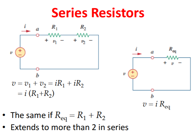
One of the basic fundamentals to simplifying and solving a circuit is to focus
on multiple resistors that have connections with one another. Depending upon
the configuration of the ladder network, the resistors in series can be
added up to simplify the resistance in that certain region of the circuit.
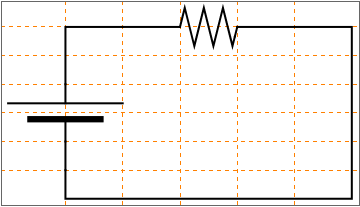
Series Resistors
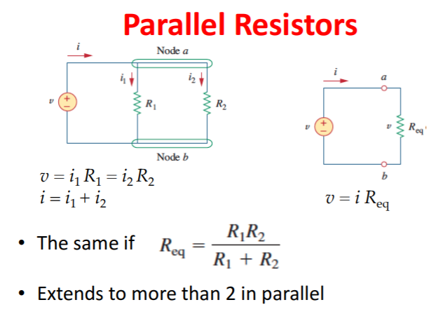
In addition, resistors in parallel can be combined by adding the inverse of all of the parallel resistances.
After the simplification of combining series and parallel resistors, there are operations in
electrical engineering that can be used to solve for other elements in the circuit. For instance,
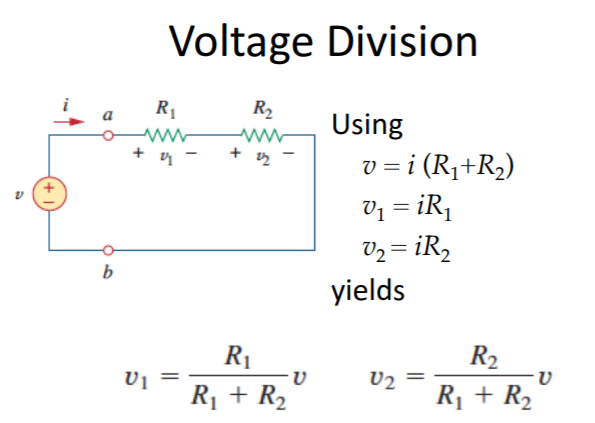
having resistors in series enables the use of voltage division. Voltage division is a procedure that
is used to solve for the voltage of a resistor (when that particular resistor is in series with
another resistor in the circuit).
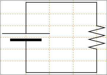
Voltage Division
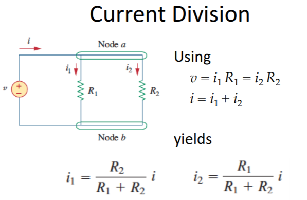
Moreover, resistors in parallel allows the use of an operation known as current division. Current
division is a function that is used to solve for the current that passes through a resistor (when that
particular resistor is connected in parallel with another resistor in the circuit).
Current Division
The input voltage (v1) and the input current (i1) in an electrical
circuit is set up in a matrix form that looks like \( \begin{bmatrix} v_1 \\ i_1
\end{bmatrix} . \) Meanwhile, the output voltage (v2) and the output current
(i2) is set up in a column vector form that equates to \( \begin{bmatrix} v_2 \\ i_2
\end{bmatrix} . \) Taking a standard electrical circuit with a linear transformation is known
as a transfer matrix, which is written as \( \begin{bmatrix} v_2 \\ i_2
\end{bmatrix} = {\bf A}\, \begin{bmatrix} v_1 \\ i_1
\end{bmatrix} . \)
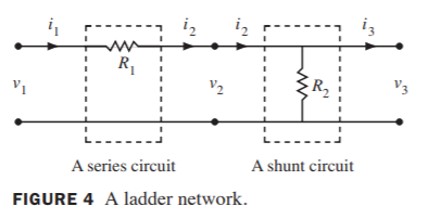
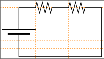
It is entirely possible that an electrical engineer could find themselves faced with solving a ladder
network, which links two circuits together that are connected in series with one another. The output
of the first circuit in the network is subsequently used as the input to the next circuit that is in
the network. In the figure pictured below, the circuit with resistor R1 is recognized as a series
circuit and the circuit with resistor R2 is recognized as a shunt circuit.
Ladder Network
Given both of these circuits, the transfer matrices for each of the respective circuits are written as
\( {\bf A}_1 = \begin{bmatrix} 1& -R_1 \\ 0&1 \end{bmatrix} \) (transfer matrix of
series circuit) and
\( {\bf A}_2 = \begin{bmatrix} 1& 0 \\ -1/R_2&1 \end{bmatrix} \) (transfer matrix of
shunt circuit). Evidently, it is possible to solve through the transfer matrix (A1
for the series circuit and A2 for the shunt circuit) that epitomizes the
figure of the ladder network that was just shown. After using an input vector x, the
transfer matrix is illustrated as
Given a transfer matrix such as \( \begin{bmatrix} 1& -8 \\ -0.5&5 \end{bmatrix} , \)
it is conceivable to compose a ladder network based off of the matrix. Using R1 and
R2 from the ladder network that is depicted on the previous page, the ladder network
would be equal to \( \begin{bmatrix} 1& -R_1 \\ -1/R_2&1+ R_1 / R_2 \end{bmatrix} =
\begin{bmatrix} 1& -8 \\ -0.5&5 \end{bmatrix} . \)
Essentially, one is a constant value from the previous transfer matrices, R1 is
equal to eight ohms, -1/R2 is equal to -.5 ohms and 1+R1/R2
is equal to five ohms. Based off of this newly designed ladder network, R2 is equal
to two ohms because one divided by .5 is equal to two ohms.
Just like in this scenario, an electrical engineer must first find out if a network like the ladder
network in figure four can be built. Assuming that the network can be created, the next step is to use
matrix factorization on the transfer matrix in order to find the matrices that are connected to smaller
circuits. The smaller circuits can then be used to compose the network or the smaller circuits may
already be a part of a configuration such as a ladder network. In some cases, the transfer matrix can
contain values that contain complex numbers. Ultimately, the goal is to try to build the network that
the electrical engineer needs while expending the least number of electrical elements.
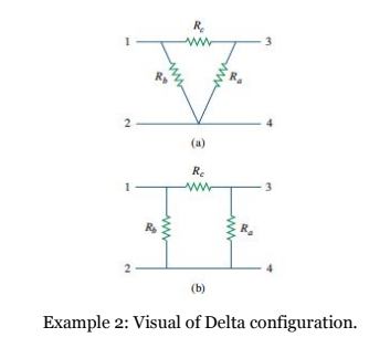
For the more daring electrical engineer, matrices can help simplify the most
complex circuits that are non-linear, like a delta-delta transformer. A
transformer is an electrical device that is designed on the basis of the
concept of magnetic coupling. It uses magnetically coupled coils to transfer
energy from one circuit to another. The transformer can be used for
“stepping up” or “stepping down” AC voltages or currents. AC stands for
alternating current and the voltage that was dealt with before
is DC (directed current). Delta configuration represents the order of components, usually two grounded
components, and one connection between them. Stating a delta-delta transformation essentially states
that they are connected together.
Not all electrical engineering problems have numbers that can be solved,
however that does not stop someone from making an equation for future use, once
other values are known. In reality, this is actually a common practice for
electrical engineers when the desired input and output is unknown.
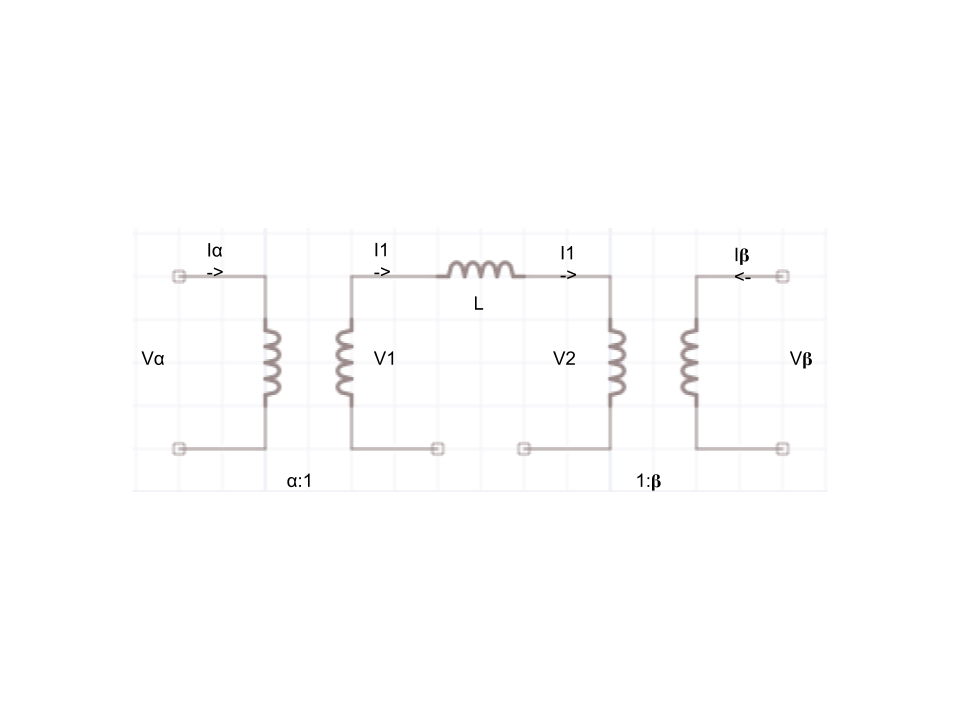
As stated before, a transformer's transfer energy comes from one circuit. Due
to power conservation, the energy that may be lost or gain is still maintained
within a ratio before the circuits, as shown below
div class = "math">
\[ -I_\beta = \beta^{-2} \left(V_\beta L \right) + \beta\alpha^{-1} \left(V_\alpha L\right)
\]
This can all be simply put into a matrix, for a quick solve once we have our
values.
\[
\left[ I_{\alpha} , I_{\beta} \right] = \left[ \alpha^{-2} L \ - (\alpha\beta )^{-1} L , \,
- (\alpha\beta )^{-1} L \ \beta^{-2} L \right]
\]
Now if even we needed to use a delta-delta transformer to step-up or step-down
and voltage or current, we can just solve for this matrix with our arguments.
In conclusion, electrical engineers calculate current flow through electrical
circuits. With the help of linear algebra, Kirchhoff's voltage law, and Ohm’s
law, one can easily solve for the value our unknown variables within a circuit.
As long as the basic assumption of network flow is true, linear algebra will
help make the problem easier to solve.
▢
This code outlines the "resistor" function. It draws a zig-zag line across a
sinusoidal function to represent a resistor within the electrical circuit. ▢
Syntax: resistor[]//at[{x, y}, Θ]
▢
This code outlines the coil function. It draws a looping line using
BezierCurve, which is a curve approximation through the given set of points.
▢
Syntax: coil[]//at[{x, y}, Θ]
▢
This code outlines the "capacitor" function. It uses the previous gap function
and lines to draw a simple capacitor. ▢
Syntax: capacitor[]//at[{x, y}, Θ]
▢
This code outlines the battery function which is used to draw a battery
at the given point and direction. It is used in conjunction with the at
function. ▢
Syntax: battery[]//at[{x, y}, \[CapitalTheta]]
▢
This code sets up the options for the plotting grid. It can be adjusted for
style purposes (the grid lines can be removed, for example. They are useful
for plotting).
▢
This code outlines the at function. It is used to set the position and
orientation of the batteries, resistors, and capacitors.
▢
Syntax: at[{x, y}, Θ]