Previously, we discussed how to solve linear vector equation Ax =
b using elimination procedure. One might expect that if the the entries
of matrix A are slightly modified, then its solution will be
closed to the original solution. Unfortunately, there exist linear systems Ax = b whose solutions are not stable under small perturbations of either b or A.
Now we pay more attension to this issue.
Example 1:
Consider the following two systems. The first one
So we see that solutions two these two systems are completely different. This
is clearly interesting, and we need to know why the behavior of solutions are
so unstable to small changes. In real life, there is almost always error in a
linear system because its values are derived from measurements with inherent
error and humans are sometimes are not accurate. We must know whether it is
possible to avoid this sensitivity to error and also what causes it.
Since we used a two-dimensional system, it can be visualized easily in the
plane. So let us solve for y in each equation.
Expand[NSolve[577 x + 880 y == 3, y]]
{{y -> 0.00340909 - 0.655682 x}}
Expand[NSolve[280 x + 427 y == 9, y]]
{{y -> 0.0210773 - 0.655738 x}}
Note that these two lines are very close to being parallel because they have
nearly identical slopes. This may be the cause of our sensitivity to slight
amounts of error since a small change in the slope of one line can move their
intersection point a great distance from the original intersection point.
■
Example 3:
We reconsider the previous example, which we rewrite using floating points to
isolate one variable:
\[
\begin{split}
0.655682 \,x + y &= 0.00340909 \\
\left( 0.655738 + E \right) x + y &= 0.0210773 ,
\end{split}
\]
where the error in the slope is E. The exact system is the one for
E = 0, and they become parallel lines when E = 0.0292836 with
no solution the system. When E = 0, the solution to the system is as
given below:
Note that if we use more decimal places and solve the equations
\[
\begin{split}
0.6556818181818181 \,x + y &= 0.003409090909090909 , \\
0.6557377049180327\, x + y &= 0.02107728337236534 ,
\end{split}
\]
we get more accurate answer:
\[
x = 316.143, \qquad y = -207.286 .
\]
The exact solution's x coordinate is given by exactSol[[1]] and
its y coordinate is given by exactSol[[2]]. For E ≠ 0,
if we denote X and Y as solutions to the approximate system,
then its distance from the exact solution is given by
\[
d = \sqrt{\left( X - exactSol[[1]] \right)^2 +
\left( Y - exactSol[[2]] \right)^2} .
\]
We ask Mathematica for help with these calculations:
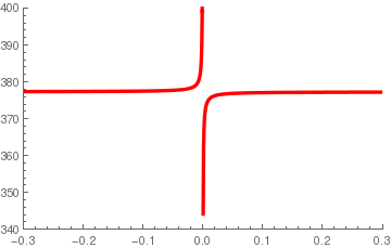
The plot of the distance between the exaxct solution and the approximate
system solutions has a vertical asymptote at E = = 0.0292836, which
is the value of E that makes the lines parallel, and so the system is
without a solution. The closer E is to this value, the larger the error.
As E moves away from 0.0292836, the error stabilizes at a value close to
278.
We are going to plot these solutions as a parametric plot in the
xy-plane to see their behavior more clearly.
■
In other words, a relative error of the order 1/200 in th edata (here, b) produces a relative error of the order 10/1 in the solution, which represents an amplification of the relative error of the order 2000.
Now, let us perturb the matrix slightly, obtaining the new system
Again, a small change in the data alters the result ratherdrastically.
■
The problem is that the matrix of the system is badly conditioned, a concept that we will now explain.
Determinant value and ill-conditioning
As some previous examples show, there exist some pathological problems of finding solutions to a linear equation A x = b that can flank the robast numerical solvers dedicated for such problems. To analyze the sensitivity of solutions to linear equations A x = b we have to employ a matrix norm ‖ · ‖ (see section), but not the determinant. It turns out that the determinant does not reflect whether matrix elements are small or large.
Its determinant is det(A) = 7×10¹⁰ and its Euclidean norm ≈ 728538. So det(A) ≫ ‖ A ‖.
Now suppose we divide the 2×2 system for our example by 1010 without changing anything in the statement of the problem. In other words, multiplying or dividing the matrix A should not lead to fundamental change. This yelds the matrix
We find det(B) = 7×10⁻¹⁰, so det(A) ≪
‖ B ‖ ≈ 0.0000728538.
Using matrix pertubation theory and carefully stady the effect a small change of the given matrix on the solution vector x + Δx looks like when when you start with A + ΔA. Following Trefethen & Bau, when we change A into A + δA, its inverse A−1 changes to A−1 + δ(A−1):
This relates an error bound on ‖Δx‖/ ‖x‖ with an error bound on ‖ΔA‖/ ‖A‖. The coefficient in front of ‖ΔA‖/ ‖A‖ tells us whether or not a small pertubation will tend to get magnified. Equation \eqref{EqSent.1} naturally leads us to introducing the condition number
When κ(A) is of order unity, we are dealing with a well-conditioned problem, i.e., a small pertubation is not amplified. Conversely, when κ(A) is large, a pertubation is typically amplified, so our problem is ill-conditioned. Crucially, this condition number involves both the matrix A and its inverse A−1. Hence, the condition number has nothing to do with the determinant. As a result, an overall scaling has no effect. For example, the condions numbers of the previously considered 2×2 matrices are