The determinant
is a special scalar-valued function defined on the set of square matrices.
Although it still has a place in many areas of mathematics and physics, our
primary application of determinants is to define eigenvalues and
characteristic polynomials for a square matrix A. It is usually
denoted as det(A), det A, or |A|. The term
determinant was first introduced by the German mathematician
Carl Friedrich Gauss in 1801.
There are various equivalent ways to define the determinant of a
square matrixA, i.e., one with the same number of rows and columns. The determinant
of a matrix of arbitrary size can be defined by the
Leibniz formula or the
Laplace formula (see next section).
Because of difficulties with motivation, intuitiveness, and simple definition, there is a tendency in exposition of linear algebra without classical involvement of determinants (see {1,2]). Since we respect both approaches, the tutorial presents several definitions of determinants. One of popular approaches is to define a determinant of a square matrix as a product of all its eigenvalues (which is a topic of next section), counting multiplicities. If the reader wants to follow this easy to remember definition, then the order of reading sections should be changed or we refer to S. Axler's textbook. It should be noted that both approaches still wait for efficient numerical algorithms. Now almost all computational software packages evaluate the determinant in O(n3) arithmetic operations by forming the LU decomposition. We start with non-constructive definition of determinant.
A functional δ from the set of all n×n matrices into
the field of scalars is called an n-linear or
multilinear
if it is a linear map of each row or each column of any
n×n matrix when the remaining n-1 rows/columns are
held fixed. Such functional is called alternating if for each square
matrix A, we have δ(A) = 0 whenever two adjacent rows (or
columns) of A are identical.
An alternating multilinear functional such that δ(I) = 1, where
I is the identity matrix, is called the determinant and is
denoted as det(A) or detA, or just |A|.
Now we give two "constructive" definitions of determinants---one is called the
Leibniz formula and another one, the Laplace cofactor expansion (next section is dedicated to this definition).
For any indexing set n = [ 1, 2, ..., n ], a
permutation of
n is a one-to-one and onto function π: n ↦ n.
An inversion in a
permutation π is any pair (i,j) ∈ n ×
n for which i < j and π(i) > &pi(j).
A permutation is called even if it has an even number of inversions and
odd otherwise.
The Leibniz formula for the determinant of an n × n matrix A is
where sgn is the sign function of permutations in the permutation groupSn, which returns +1 and −1 for even and odd permutations, respectively.
Here the sum is computed over all permutations σ of the set {1, 2, …, n}.
A permutation is a function that reorders this set of integers. The value in
the i-th position after the reordering σ is denoted by σi.
The Laplace expansion, named after Pierre-Simon Laplace, also called cofactor expansion, is an expression for the determinant |A| of an n × n matrix A that is a weighted sum of the determinants of n sub-matrices of A, each of size (n−1) × (n−1).
The Laplace expansion (which we discuss in the next section) as well as the
Leibniz formula are of theoretical interest as one of several ways to
view the determinant, but not for practical use in determinant computation.
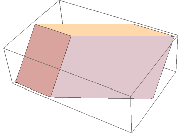
Determinants are used to determine the volumes of parallelepipeds formed by
n vectors in n-dimensional Euclidean space. In 2 and 3
dimensional cases, the determinant is the area of parallelogram and the volume
of parallelepiped, respectively. We plot them with Mathematica
The n-volume of an n-parallelepiped formed by n vectors
in
ℝn is the absolute value of the determinant of these n
vectors. When a square matrix A is considered as a transformation
ℝn ↦ ℝn, the absolute value of its
determinant is called the magnification factor because it the volume of
the image of the unit n-cube.
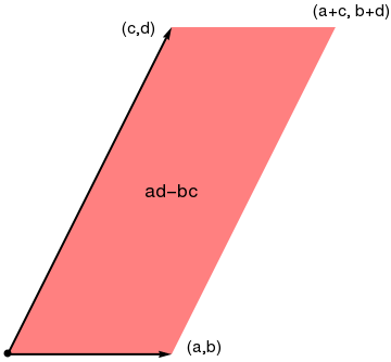
The Leibniz formula for the determinant of a 2 × 2 matrix is
If the matrix entries are real numbers, the matrix A can be used to
represent two linear maps: one that maps the standard basis vectors to the
rows of A, and one that maps them to the columns of A. In either
case, the images of the basis vectors form a parallelogram that represents the
image of the unit square under the mapping. The parallelogram defined by the
rows of the above matrix is the one with vertices at (0, 0), (a, b), (a + c, b + d), and (c, d), as shown in the accompanying diagram.
The formula for the determinant of a 3 × 3 matrix is
As we see from the above formula, the determinant of 3×3 matrix A
can be found by augmenting to A its first two columns and then
summing the three products down the diagonal from upper left to lower right
followed by subtracting the three products up the three diagonals from lower
left to upper right. Unfortunately, this algorithm does not generalize to
larger matrices.
A = {{a, b, c}, {d, e, f}, {g, h, i}};
Join[A, A[[All, 1 ;; 2]], 2] // MatrixForm
In general, the determinant of an n × n matrix contains
n! terms, half of them come up with positive sign and another half are
negative.
A square matrix is called upper triangular (lower triangular) if all the entries below
the main diagonal are
zero (correspondingly, if all the entries above the main diagonal are zero).
A square matrix is called triangular if it is either upper or lower
triangular.
\( \det \left( k{\bf A} \right) =
k^n \det \left( {\bf A} \right) \) for a constant k.
If A is a triangular matrix, i.e. ai,j = 0 whenever
i > j or, alternatively, whenever i < j,
then its determinant equals the product of the diagonal entries.
If B is a matrix resulting from an n × n matrix A by elementary
row operation of swapping two rows, then det(B) = -det(A).
If B is a matrix resulting from an n × n matrix A by elementary
row operation of multiplying by a scalar k any row, then
det(B) = k det(A).
If B is a matrix resulting from an n × n matrix A by elementary
row operation of multiplying by a scalar k any row and adding to
another row, then det(B) = det(A).
If we can transform a general square matrix A into a new triangular
matrix T without changing the value (or as alternative, with simple and
clear its modification), then we would have a method of computing its determinant. The way to change a general square matrix into an upper triangular matrix is through the three elementary row operations and their corresponding matrix multiplication counterparts. A matrix that is similar to a triangular matrix is referred to as triangularizable. Every matrix over the field of complex numbers ℂ is triangularizable, but not every real-valued matrix.
Its determinant contains 4! = 24 terms, each is a product of entries from
A taken one from each row and each column; so using the Laplace
expansion, we get
Now it is time to make the process of converting a matrix to upper triangular
a bit more automated using Mathematica. This can be done with two
steps: first we use subroutine PivotDown that annihilates all entries
in a column below a desired location. The second function, DetbyGauss
uses PivotDown to convert a matrix to upper triangular, and when
possible, do it without row exchange.
PivotDown[m_, {i_, j_}, oneflag_: 0] :=
Block[{k}, If[m[[i, j]] == 0, Return[m]];
Return[Table[
Which[k < i, m[[k]], k > i, m[[k]] - m[[k, j]]/m[[i, j]] m[[i]],
k == i && oneflag == 0, m[[k]] , k == 1 && oneflag == 1,
m[[k]]/m[[i, j]] ], {k, 1, Length[m]}]]]
Applying the subroutine DetbyGauss, we obtain its triangulation:
DetbyGauss[A]
there were 1 row swap(s) \( \begin{pmatrix}
3&2&-1&4 \\ 0&2&5&-1 \\ 0&0&6&- \frac{5}{3} \\ 0&0&0&-\frac{1}{18}
\end{pmatrix} \)
Multiplying the diagonal elements, we get the value of the determinant for the
upper triangular matrix to be -2. However, since there was one swap, we have to
multiply the latter by -1, which yields the correct answer: 2.
■