Vectors

Linear algebra is primarily concerned with two types of mathematical objects: matrices and vectors. Moreover, these objects are common in all branches of science related to physics, engineering, and economics. Since matrices are build from vectors, this section focuses on the latter by presenting basic vector terminology and corresponding concepts. Fortunately, we have proper symbols for their computer manipulations.

Important properties of linear systems can be described with concept and notation of vectors. As a motivating example, let us consider a system of three equations

\begin{align*} 2\,x_1 -3\,x_2 + x_3 &= 3, \\ -x_1 + 2\,x_2 - 4\,x_3 &= 5 , \\ 3\, x_1 + 4\,x_2 - 2\, x_3 &= 3. \end{align*}
We rewrite this system in columns as
\[ \begin{bmatrix} 2\,x_1 \\ - x_1 \\ 3\,x_1 \end{bmatrix} + \begin{bmatrix} -3\, x_2 \\ \phantom{-}2\, x_2 \\ \phantom{-}4\,x_2 \end{bmatrix} + \begin{bmatrix} \phantom{-1}x_3 \\ -4\, x_3 \\ -2\, x_3 \end{bmatrix} = \begin{bmatrix} 3 \\ 5 \\ 3 \end{bmatrix} \]
because we know how to operate with numbers. So we assume that we can add these columns by adding corresponding components. Taking out common multiples in each column, we get
\[ x_1 \begin{bmatrix} \phantom{-}2 \\ -1 \\ \phantom{-}3 \end{bmatrix} + x_2 \begin{bmatrix} -3 \\ \phantom{-}2 \\ \phantom{-}4 \end{bmatrix} + x_3 \begin{bmatrix} \phantom{-}1 \\ -4 \\ -2 \end{bmatrix} = \begin{bmatrix} 3 \\ 5 \\ 3 \end{bmatrix} . \]
The expression in the left-hand side is known as a linear combination---it is obtained by adding two or more vectors that are multiplied by scalar values. Calling each column a vector, we denote them with lower case letter written in bold font:
\[ {\bf u}_1 = \begin{bmatrix} \phantom{-}2 \\ -1 \\ \phantom{-}3 \end{bmatrix} , \quad {\bf u}_2 = \begin{bmatrix} -3 \\ \phantom{-}2 \\ \phantom{-}4 \end{bmatrix} , \quad {\bf u}_3 = \begin{bmatrix} \phantom{-}1 \\ -4 \\ -2 \end{bmatrix} , \qquad {\bf b} = \begin{bmatrix} 3 \\ 5 \\ 3 \end{bmatrix} . \]
The entries of vectors are integers, but they are suitable only for class presentations by lazy instructors like me. In real life, the set of integers ℤ appears mostly in kindergarten. Therefore, vector entries could be any numbers, for instance, real numbers denoted by ℝ, or complex numbers ℂ. However, humans and computers operate only with rational numbers ℚ as approximations of fields ℝ or ℂ. Although the majority of our presentations involves integers for simplicity, the reader should understand that they can be replaced by arbitrary numbers from either ℝ or ℂ or ℚ. When it does not matter what set of numbers can be utilized, which usually the case, we denote them by 𝔽 and the reader could replace it with any field (either ℝ or ℂ or ℚ).

The term vector appears in a variety of mathematical and engineering contexts, which we will discuss in Part3 (Vector Spaces). There is no universal notation for vectors because of diversity of their applications. Until then, vector will mean an ordered set (list) of numbers. Generally speaking, concept of vector may include infinite sequence of numbers or other objects. However, in this part of tutorial, we consider only finite lists. There are many ways to represent vectors including columns, rows, or just n-tuples as elements of Cartesian product of real numbers:

\begin{equation} \label{EqVector.1} {\bf v} = (v_1 , v_2 , \ldots , v_n ) \in \mathbb{R} \times \mathbb{R} \times \cdots \times \mathbb{R} . \end{equation}
In many cases, it is convenient to distinguish column vectors from row vectors upon introducing the following notations. In physics, Dirac's bra-ket notation is also widely use, which we utilize in later chapters (Part 3 and Part 5).
The set of all real or complex n-tuples is denoted by ℝ × ℝ ×⋯× ℝ or ℂ × ℂ ×⋯× ℂ, respectively, as they are products of n real or complex number sets. The set of all real column vectors is denoted by ℝn:
\[ \mathbb{R}^n = \left\{ \begin{bmatrix} x_1 \\ x_2 \\ \vdots \\ x_n \end{bmatrix} : x_1, x_2 , \ldots , x_n \in \mathbb{R} \right\} . \]
Similarly, the set of all complex n-column vectors is denoted by ℂn:
\[ \mathbb{C}^n = \left\{ \begin{bmatrix} z_1 \\ z_2 \\ \vdots \\ z_n \end{bmatrix} : z_1, z_2 , \ldots , z_n \in \mathbb{C} \right\} . \]
Sometimes, the the vector space of all n-row vectors are denoted by ℝn or ℂn, depending on entries being real or complex.
For our purposes, it is convenient to represent vectors as columns. This allows us to rewrite the given system of algebraic equations in compact form:
\[ x_1 {\bf u}_1 + x_2 {\bf u}_2 + x_3 {\bf u}_3 = {\bf b} . \]
In general, a system of m linear equations
\begin{align} a_{1,1} x_1 + a_{1,2} x_2 + \cdots + a_{1,n} x_n &= b_1 , \notag \\ a_{2,1} x_1 + a_{2,2} x_2 + \cdots + a_{2,n} x_n &= b_2 , \label{EqVector.2} \\ \ddots \qquad\qquad & \qquad \vdots \notag \\ a_{m,1} x_1 + a_{m,2} x_2 + \cdots + a_{m,n} x_n &= b_m , \notag \end{align}
with n unknowns, x1, x2, … , xn, can be similarly rewritten as a linear combination
\begin{equation} \label{EqVector.3} x_1 {\bf u}_1 + x_2 {\bf u}_2 + \cdots + x_n {\bf u}_n = {\bf b} . \end{equation}
of column vectors
\begin{equation} \label{EqVector.4} {\bf u}_1 = \begin{bmatrix} a_{1,1} \\ a_{2,1} \\ \vdots \\ a_{m,1} \end{bmatrix} , \quad {\bf u}_2 = \begin{bmatrix} a_{1,2} \\ a_{2,2} \\ \vdots \\ a_{m,2} \end{bmatrix} , \quad \cdots \quad {\bf u}_n = \begin{bmatrix} a_{1,n} \\ a_{2,2} \\ \vdots \\ a_{m,n} \end{bmatrix} , \qquad {\bf b} = \begin{bmatrix} b_{1} \\ b_{2} \\ \vdots \\ b_{m} \end{bmatrix} . \end{equation}
The compact form \eqref{EqVector.3} of the linear system of equations \eqref{EqVector.2} tells us that we can add vectors by adding their components
\[ {\bf u} + {\bf v} = \begin{bmatrix} u_1 \\ u_2 \\ \vdots \\ u_n \end{bmatrix} + \begin{bmatrix} v_1 \\ v_2 \\ \vdots \\ v_n \end{bmatrix} = \begin{bmatrix} u_1 + v_1 \\ u_2 + v_2 \\ \vdots \\ u_n + v_n \end{bmatrix} \]
and multiply by a number, say k as
\[ k\,{\bf u} = k \begin{bmatrix} u_1 \\ u_2 \\ \vdots \\ u_n \end{bmatrix} = \begin{bmatrix} k\,u_1 \\ k\,u_2 \\ \vdots \\ k\,u_n \end{bmatrix} . \]
The number k in ku is called a scalar: it is written in the lightface type to distinguish it from the boldface vector u. Note that components of vector u are also written in the lightface type because they are numbers that we call scalars. How to operate with numbers (scalars) everybody knows from school: they can be added/subtracted and multiplied/divided by nonzero number.

Remember that the form of vector representation as columns, rows, or n-tuples (parentheses and comma notation) depends on you. However, you must be consistent and use the same notation for addition or scalar multiplication. You cannot add a column vector and a row vector:
\[ \begin{bmatrix} 1 \\ 2 \end{bmatrix} + \left[ 1, \ 2 \right] \qquad{\bf wrong!} \]
because they have different structures. In physics, row vectors are usually called bra vectors and column vectors are named ket vectors. Also, you cannot manipulate row vectors and n-tuples:
\[ \left[ 1, \ 2,\ 3 \right] + \left( 1, \ 2,\ 3 \right) \qquad{\bf wrong!} \]
because (1, 2, 3) ∈ ℝ×ℝ×ℝ, but [1 2 3] is 1×3 matrix. Of course, all three sets ℝ×ℝ×ℝ, ℝ³, and ;ℝ₃ are equivalent since all are just descriptions (depending on humans) of the same vectors (nature).

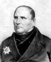
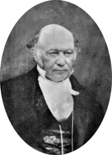
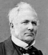
   Giusto Bellavitis  Michail Ostrogradsky      William Hamilton

The concept of vector, as we know it today, evolved gradually over a period of more than 200 years. The Italian mathematician, senator, and municipal councilor Giusto Bellavitis (1803--1880) abstracted the basic idea in 1835. The idea of an n-dimensional Euclidean space for n > 3 appeared in a work on the divergence theorem by the Russian mathematician Michail Ostrogradsky (1801--1862) in 1836, in the geometrical tracts of Hermann Grassmann (1809--1877) in the early 1840s, and in a brief paper of Arthur Cayley (1821--1895) in 1846. Unfortunately, the first two authors were virtually ignored in their lifetimes. In particular, the work of Grassmann was quite philosophical and extremely difficult to read. The term vector was introduced by the Irish mathematician, astronomer, and mathematical physicist William Rowan Hamilton (1805--1865) as part of a quaternion.

Vectors can be described also algebraically. Historically, the first vectors were Euclidean vectors that can be expanded through standard basic vectors that are used as coordinates. Then any vector can be uniquely represented by a sequence of scalars called coordinates or components. The set of such ordered n-tuples is denoted by \( \mathbb{R}^n . \) When scalars are complex numbers, the set of ordered n-tuples of complex numbers is denoted by \( \mathbb{C}^n . \) Motivated by these two approaches, we present the general definition of vectors.

Example 1: For given vectors u = (−2, 1) and v = (1, 2), find 3u + (−2)v.

Rewriting vectors u and v in column form, we have

\[ 3{\bf u} + (-2){\bf v} = 3 \begin{bmatrix} -2 \\ \phantom{-}1 \end{bmatrix} + (-2) \begin{bmatrix} 1 \\ 2 \end{bmatrix} = \begin{bmatrix} -6 - 2 \\ 3 -4 \end{bmatrix} = \begin{bmatrix} -8 \\ -1 \end{bmatrix} . \]
Example 2: For given two vectors
\[ {\bf u} = \begin{bmatrix} \phantom{-}1 \\ -2 \\ \phantom{-}3 \end{bmatrix} \qquad \mbox{and} \qquad {\bf v} = \begin{bmatrix} \phantom{-}3 \\ -4 \\ \phantom{-}2 \end{bmatrix} , \]
represent vector
\[ {\bf b} = \begin{bmatrix} -5 \\ \phantom{-}6 \\ -1 \end{bmatrix} \]
as a linear combination of vectors u and v. So we need to find x₁ and x₂ such that
\[ x_1 {\bf u} + x_2 {\bf v} = {\bf b} = \begin{bmatrix} -5 \\ \phantom{-}6 \\ -1 \end{bmatrix} . \tag{2.1} \]
The definition of scalar multiplication and vector addition lead to
\[ x_1 \begin{bmatrix} \phantom{-}1 \\ -2 \\ \phantom{-}3 \end{bmatrix} + x_2 \begin{bmatrix} \phantom{-}3 \\ -4 \\ \phantom{-}2 \end{bmatrix} = \begin{bmatrix} -5 \\ \phantom{-}6 \\ -1 \end{bmatrix} , \]
which is the same as
\[ \begin{bmatrix} x_1 + 3 x_2 \\ -2 x_1 - 4 x_2 \\ 3 x_1 + 2 x_2 \end{bmatrix} =\begin{bmatrix} -5 \\ \phantom{-}6 \\ -1 \end{bmatrix} . \tag{2.2} \]
The vectors on the right and left sides of (2.2) are equal if and only if their corresponding entries are both equal. That is, x₁ and x₂ make the vector equation (2.1) true if and only if x₁ and x₂ satisfy the system
\[ \begin{split} x_1 + 3 x_2 &= -5 , \\ -2 x_1 -4 x_2 &= 6 , \\ 3x_1 + 2 x_2 &= 2 . \end{split} \tag{2.3} \]
To solve this system of equation, we apply row reduction to the augmented matrix
\[ \begin{bmatrix} \phantom{-}1 & \phantom{-}3 & -5 \\ -2 & -4 & \phantom{-}6 \\ \phantom{-}3 & \phantom{-}2 & -1 \end{bmatrix} \ \sim \ \begin{bmatrix} 1 & \phantom{-}3 & -5 \\ 0 & \phantom{-}2 & -4 \\ 0 & -7 & 14 \end{bmatrix} \ \sim \ \begin{bmatrix} 1 & 3 & -5 \\ 0 & 2 & -4 \\ 0 & 0 & \phantom{-}0 \end{bmatrix} \]
The solution of (2.3) is x₁ = 1 and x₂ = −2. Hence b is a linear combination of u and v with weights x₁ = 1 and x₂ = −2. That is,
\[ (1) \begin{bmatrix} \phantom{-}1 \\ -2 \\ \phantom{-}3 \end{bmatrix} + (-2) \begin{bmatrix} \phantom{-}3 \\ -4 \\ \phantom{-}2 \end{bmatrix} = \begin{bmatrix} -5 \\ \phantom{-}6 \\ -1 \end{bmatrix} . \]

  1. Compute uv and 3u −2v ---> \[ {\bf u} = \begin{bmatrix} -2 \\ \phantom{-}1 \end{bmatrix} , \quad {\bf v} = \begin{bmatrix} 3 \\ 2 \end{bmatrix} \qquad\mbox{and} \qquad {\bf u} = \begin{bmatrix} \phantom{-}1 \\ -1 \end{bmatrix} , \quad {\bf v} = \begin{bmatrix} \phantom{-}4 \\ -3 \end{bmatrix} . \]
  2. Write system of equations that is equivalent to the given vector equation.
    1. \[ x_1 \begin{bmatrix} \phantom{-}3 \\ -4 \end{bmatrix} + x_2 \begin{bmatrix} -1 \\ -2 \end{bmatrix} + x_3 \begin{bmatrix} \phantom{-}5 \\ -2 \end{bmatrix} = \begin{bmatrix} \phantom{-}1 \\ -1 \end{bmatrix}; \]
    2. \[ x_1 \begin{bmatrix} 3 \\ 0 \\ 2 \end{bmatrix} + x_2 \begin{bmatrix} -1 \\ \phantom{-}3 \\ \phantom{-}5 \end{bmatrix} + x_3 \begin{bmatrix} -2 \\ \phantom{-}7 \\ \phantom{-}2 \end{bmatrix} = \begin{bmatrix} 5 \\ 1 \\ 3 \end{bmatrix}; \]
    3. \[ x_1 \begin{bmatrix} 2 \\ 1 \\ 7 \end{bmatrix} + x_2 \begin{bmatrix} \phantom{-}3 \\ -2 \\ -5 \end{bmatrix} + x_3 \begin{bmatrix} \phantom{-}4 \\ -6 \\ \phantom{-}1 \end{bmatrix} = \begin{bmatrix} -5 \\ -4 \\ \phantom{-}2 \end{bmatrix} . \]
  3. Given \( \displaystyle {\bf u} = \begin{bmatrix} 2 \\ 1 \\ 3 \end{bmatrix} , \ {\bf v} = \begin{bmatrix} \phantom{-}3 \\ -1 \\ -5 \end{bmatrix} , \quad\mbox{and} \quad {\bf b} = \begin{bmatrix} -5 \\ 5 \\ h \end{bmatrix} . \) For what value of h is b a linear combination of vectors u and v?
  4. Given \( \displaystyle {\bf u} = \begin{bmatrix} 4 \\ 3 \\ 1 \end{bmatrix} , \ {\bf v} = \begin{bmatrix} \phantom{-}2 \\ -2 \\ -3 \end{bmatrix} , \quad\mbox{and} \quad {\bf b} = \begin{bmatrix} 8 \\ h \\ 9 \end{bmatrix} . \) For what value of h is b a linear combination of vectors u and v?
  5. Rewrite the system of equations in a vector form
    \[ \begin{split} 2x_1 - 3 x_2 + 7 x_3 &= -1 , \\ -5 x_1 -2 x_2 - 3 x_3 &= 2 , \\ 3x_1 + 2 x_2 + 4 x_3 &= 3 . \end{split} \]
  6. Let \( \displaystyle {\bf u} = \begin{bmatrix} 3 \\ 1 \end{bmatrix} , \ {\bf v} = \begin{bmatrix} \phantom{-}2 \\ -2 \end{bmatrix} , \quad\mbox{and} \quad {\bf b} = \begin{bmatrix} h \\ k \end{bmatrix} . \) Show that the linear equation xu + xv = b has a solution for any values of h and k.
  7. Mark each statement True or False.
    1. Another notation for the vector (1, 2) is \( \displaystyle \begin{bmatrix} 1 \\ 2 \end{bmatrix} . \)
    2. An example of a linear combination of vectors u and v is 2v.
    3. Any list of of six complex numbers is a vector in ℂ6.
    4. The vector 2v results when a vector v + u is added to the vector vu.
    5. The solution set of the linear system whose augmented matrix is [ a1 a2 a3 b ] is the same as the solution set of the vector equation xa₁ + xa₂ + xa₃ = b.
  1. Vector addition
  2. Tea
  3. Milk