
Introduction to Linear Algebra
Systems of Linear Equations
- Introduction
- Linear systems
- Vectors
- Linear combinations
- Matrices
- Planes in ℝ³
- Reduced Row-Echelon Form
- Equation A x = b
- Sensitivity of solutions
- Linear independence
- Plane transformations
- Space transformations
- Linear transformations
- Affine maps
- Exercises
- Answers
Matrix Algebra
- Introduction
- Manipulation of matrices
- Partitioned matrices
- Block matrices Matrix operators
- Determinants
- Cofactors
- Cramer's rule
- Equivalent matrices
- Elimination: A = L U
- PLU factorization
- Reflection
- Givens rotation
- Special matrices
- Exercises
- Answers
Vector Spaces
- Introduction
- Motivation
- Vector spaces
- Bases
- Dimension
- Coordinate systems
- Change of basis
- Linear transformations
- Matrix transformations
- Compositions
- Isomorphisms
- Dual transformations
- Direct sums
- Quotient spaces
- Rank
- Solving A x = b
- Exercises
- Answers
Eigenvalues, Eigenvectors
- Introduction
- Characteristic polynomials
- Companion matrix
- Algebraic and geometric multiplicities
- Minimal polynomials
- Eigenspaces
- Where are eigenvalues?
- Eigenvalues of A B and B A
- Generalized eigenvectors
- Similarity
- Diagonalizability
- Self-adjoint operators
Euclidean Spaces
- Introduction
- Dot product
- Bilinear transformations
- Inner product
- Norm and distance
- Matrix norms
- Dual norms
- Dual transformations
- Examples of transformations
- Orthogonality
- Gram--Schmidt Process
- Orthogonal sets
- Self-adjoint Matrices
- Unitary matrices
- Projection operators
- QR-decomposition
- Least Square Approximation
- Quadratic forms
- Exercises
- Answers
Matrix Decompositions
- Introduction
- Symmetric matrices
- LU-decomposition
- QR-decomposition
- Cholesky decomposition
- Schur decomposition
- Positive matrices
- Roots
- Polar factorization
- Spectral decomposition
- Singular values
- SVD <
- Pseudoinverse
- Exercises
- Answers
Applications
- GPS problem
- Poisson equation
- Graph theory
- Error correcting codes
- Electric circuits
- Markov chains
- Cryptography
- Wave-length transfer matrix
- Computer graphics
- Linear Programming
- Hill's determinant
- Fibonacci matrices
- Discrete dynamic systems
- Discrete Fourier transform
- Fast Fourier transform
- Curve fitting
Functions of Matrices
- Introduction
- Diagonalization
- Sylvester formula
- The Resolvent method
- Polynomial interpolation
- Positive matrices
- Roots <
- Pseudoinverse
- Exercises
- Answers
Miscellany
- Circles along curves
- TNB frames
- Tensors
- Tensors in ℝ³
- Tensors & Mechanics
- Differential forms
- Calculus
- Vector representations
- Matrix representations
- Change of basis
- Orthonormal Diagonalization
- Generalized inverse
- Differential forms
Preliminaries
- Complex Number Operations
- Sets
- Polynomials
- Polynomials and Matrices
- Computer solves Systems of Linear Equations
- Location of Eigenvalues
- Power Method
- Iterative Method
- Similarity and Diagonalization
Glossary
Reference

This Book is licensed under Creative Commons Attribution-NonCommercial-NoDerivs 3.0 Unported License
Plane Transformations
This section is devoted to illustrations of linear transformations on the plane and three-dimensional space using square matrices. This may help you to develop a geometric understanding of matrices and their relationship to coordinate space transformations in general. Every square matrix can be considered as an operator that acts on column vectors from left-to-right, with output also written as column vector. Then each linear transformation ℝn ⇾ ℝn is identified by a square n×n matrix A, and vise versa. When ℝn is identified with the space of column vectors, ℝn×1, a linear transformation in it is generated by matrix multiplication from left: A x, where x is an arbitrary column vector, x ∈ ℝn×1.
Plane transformations can be classified as reflections, contractions/expansions, shears, rotations, and projections (that is a topic of another section). The following subsections give appropriate terminologies for such transformations. The difference between matrix multiplication A x and corresponding linear transformation TA : ℝ² ⇾ ℝ² is merely a matter of notation. Therefore, we can classify matrices instead of as linear maps. We mention the following properties of matrix transformations:
- linearity,
- closed under composition,
- associativity,
- not commutative,
- applied left-to-right.
We demonstrate linear transformations acting on a house that we place at the original, which is the corner of {0,0} in the Cartesian two-dimensional plane. Matrix algebra is used to move this house with each transformation having the same common corner at the origin. The first is not a transformation but the baseline beginning point which will be transformed as we proceed. The object of choice is a parallelogram as transformation of the vector points is all that is required to make the change we desire.
Clear[house]; house[trans_ : {{1, 0}, {0, 1}}, label_ : "House in Quadrant I"] := Module[{para, tri, door}, para = Parallelogram[{0, 0}, trans]; tri = Triangle[{trans[[2]], {trans[[1, 1]], trans[[2, 2]]}, {.5*trans[[1, 1]], 1.5*trans[[2, 2]]}}]; door = Parallelogram[.4* trans[[1]], {.2*trans[[1]], .5 trans[[2]]}]; Graphics[{Blue, para, Red, tri, White, door}, Axes -> True, PlotLabel -> label, PlotRange -> {{-3, 3}, {-3, 3}}] ] houseNE = house[]

Uniform scale

|
\[ \begin{bmatrix} 1.5 & 0 \\ 0 & 1.5 \end{bmatrix} \] |

|
|
|
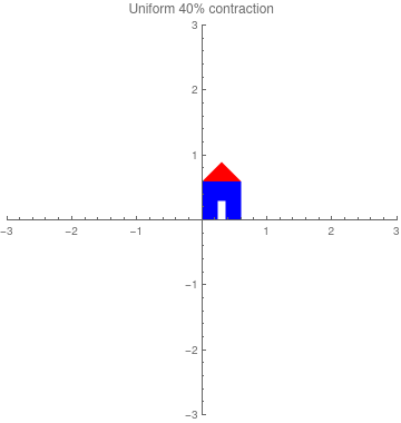
\[ \begin{bmatrix} 0.6 & 0 \\ 0 & 0.6 \end{bmatrix} \] |
|
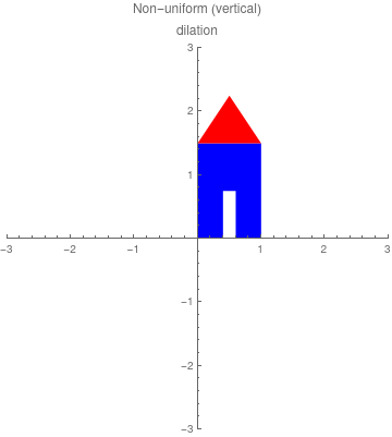
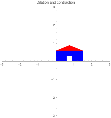
Nonuniform scale
|
|
\[ \begin{bmatrix} 1 & 0 \\ 0 & 1.5 \end{bmatrix} \] |
|
|
|
\[ \begin{bmatrix} 1.5 & 0 \\ 0 & 1 \end{bmatrix} \] |

|
|
|
\[ \begin{bmatrix} 1.5 & 0 \\ 0 & 2 \end{bmatrix} \] |

|
|
|
\[ \begin{bmatrix} 1 & 0 \\ 0 & 0.6 \end{bmatrix} \] |

|
|
|
\[ \begin{bmatrix} 0.6 & 0 \\ 0 & 1 \end{bmatrix} \] |

|
|
|
\[ \begin{bmatrix} 1.5 & 0 \\ 0 & 0.6 \end{bmatrix} \] |
|
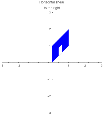
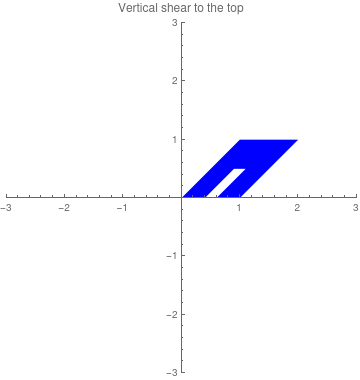
Shear Map
The code for the roof does not play well with the shear transform, so we dispense with the roof below, leaving only a door to remind us we started with a house. There are a number of ramifications to this worth mentioning before continuing. First, the roof is a triangle. Matrix algebra is about matrices, which are by their nature rectangles, not triangles. The reason the door survives in the illustration is that it is a rectangle, like the base. Second, when the base of the house is a rectangle the roof "follows" the base in the code, which is not true when the base is a non-rectangular parallelogram. This respects the reality that all rectangles are parallelograms but the converse is not true. Third, the house is a metaphor, an abstraction to advance the pedagogy in connection with linear algebra. We must be careful taking pedagogy into the real world. Put a roof on a base that is a tilted parallelogram and watch the house fall down to prove the importance of having the load orthogonal to its support in the real world where gravity matters.
|
|
\[ \begin{bmatrix} 1 & 1 \\ 0 & 1 \end{bmatrix} \] |
|
|
|
\[ \begin{bmatrix} 1 & -1 \\ 0 & \phantom{-}1 \end{bmatrix} \] |

|
|
|
\[ \begin{bmatrix} 1 & 0 \\ 1 & 1 \end{bmatrix} \] |
|
|
|
\[ \begin{bmatrix} \phantom{-}1 & 0 \\ -1 & 1 \end{bmatrix} \] |

|
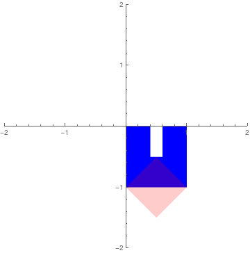
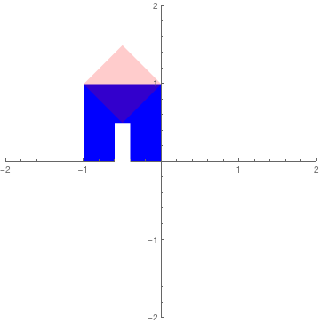
Reflection
The first three transformations can be considered as a special case of nonuniform scale.
Below, the first is the Identity Matrix and the last three are the reflection matrices.
|
|
\[ \begin{bmatrix} 1 & \phantom{-}0 \\ 0 & -1 \end{bmatrix} \] |
|
|
|
\[ \begin{bmatrix} -1 & \phantom{-}0 \\ \phantom{-}0 & -1 \end{bmatrix} \] |

|
|
|
\[ \begin{bmatrix} -1 & 0 \\ \phantom{-}0 & 1 \end{bmatrix} \] |
|
|
|
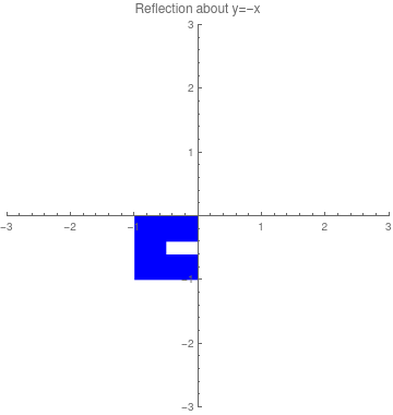
\[ \begin{bmatrix} \phantom{-}0 & -1 \\ -1 & \phantom{-}0 \end{bmatrix} \] |
|
|
|
\[ \begin{bmatrix} 0 & 1 \\ 1 & 0 \end{bmatrix} \] |
|
|
|
\[ \frac{1}{2} \begin{bmatrix} 1 & \sqrt{3} \\ \sqrt{3} & -1 \end{bmatrix} \] |
|
Rotation
For example, to generate a rhombus with vertices (0, 0), (1, 1), (0, 2), and (1, −1), we store the pairs as columns of a matrix: \[ {\bf T} = \begin{bmatrix} 0 & 1 & 0 & 1 & 0 \\ 0 & 1 & 2 & -1 & 0 \end{bmatrix} . \] An additional copy of the vertex (0, 0) is stored in the last column of T so that the previous point (1, −1) will be connected back to (0, 0) [see Figure 4.2.3(a)].

|
Leon, page 205, Figure 4.2.3
|
We can transform a figure by changing the positions of the vertices and then redrawing the figure. If the transformation is linear, it can be carried out as a matrix multiplication. Viewing a succession of such drawings will produce the effect of animation. The four primary geometric transformations that are used in computer graphics are as follows:
- Dilations and contractions. A linear operator of the form \[ T({\bf x}) = c\,{\bf x} \] is a dilation if c > 1 and a contraction if 0 < c < 1. The operator T is represented by the matrix cI, where I is the 2 × 2 identity matrix. A dilation increases the size of the figure by a factor c > 1, and a contraction shrinks the figure by a factor c < 1. Figure 4.2 shows a dilation by a factor of 1.5 of the rhombus stored in the matrix T.
-
Reflections about an axis. If Tx is a transformation that reflects a vector x
about the x-axis, then Tx is a linear operator and hence it can be represented
by a 2 × 2 matrix A. Since
\[
T_x ({\bf e}_1 ) = {\bf e}_1 \qquad \mbox{and} \qquad T_x ({\bf e}_2 ) = -{\bf e}_2 ,
\]
it follows that
\[
{\bf A} = \begin{bmatrix} 1 & \phantom{-}0 \\ 0 & -1 \end{bmatrix} .
\]
Similarly, if Ty is the linear operator that reflects a vector about the y-axis, then Ty is represented by the matrix \[ \left[ T_y \right] = \begin{bmatrix} -1 & 0 \\ \phantom{-}0 & 1 \end{bmatrix} . \] Figure 4.2.3(c) shows the image of the rhombus after a reflection about the y-axis.
Rhombus defined by T. Leon, page 205, Figure 4.2.3
Rhombus reflected by y. Leon, page 205, Figure 4.2.3 -
Rotations. Let T be a transformation that rotates a vector about the origin by
an angle θ in the counterclockwise direction. We saw in Example ???? that T is a
linear operator and that T(x) = A x, where
\[
{\bf A} = \begin{bmatrix} \cos\theta & -\sin\theta \\ \sin\theta & \phantom{-}\cos\theta \end{bmatrix} .
\]
Figure 4.2.3(d) shows the result of rotating the triangle T by 60 ◦ in the
counterclockwise direction.
Rhombus rotated by 60°. Leon, page 205, Figure 4.2.3 - Translations. A translation by a vector a is a transformation of the form \[ T({\bf x}) = {\bf x} + {\bf a} . \] If a ≠ = 0, then T is not a linear transformation and hence T cannot be represented by a 2 × 2 matrix. However, in computer graphics it is desirable to do all transformations as matrix multiplications. The way around the problem is to introduce a new system of coordinates called homogeneous coordinates.
- An expansion along a coordinate axis.
- A compression along a coordinate axis.
- A shear along a coordinate axis.
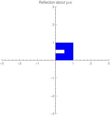
- A reflection along y = x.
- A reflection about a coordinate axis.
- A compression or expansion along a coordinate axis followed by reflection about a coordinate axis.
The last matrix represents a reflection about y = x.
|
|
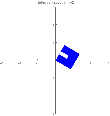
\[ \begin{bmatrix} 1 & 0 \\ \frac{3}{2} & 1 \end{bmatrix} \] |
|
These three successive row operations can be performed by multiplyingA on the left successively by \[ {\bf E}_1 = \begin{bmatrix} 0 & 1 \\ 1 & 0 \end{bmatrix} , \qquad {\bf E}_2 = \begin{bmatrix} \frac{2}{3} & 0 \\ 0 & 1 \end{bmatrix} , \qquad {\bf E}_3 = \begin{bmatrix} 1 & -\frac{2}{3} \\ 0 & \phantom{-}1 \end{bmatrix} . \] Inverting these matrices, we get
- shearing by factor of ⅔ in the abscissa direction;
- expanding by a factor of 3/3 in the x-direction;
- reflecting about the line y = x.

|

|

|
Orthogonal projection
- Find the standard matrix for a linear transformation T: ℝ² ↦ ℝ² that first reflects points through the horizontal x1-axis and then reflects points through the line x1 = x2.
- Find the standard matrix for a linear transformation T: ℝ² ↦ ℝ² that first rotates points through -3π/4 radian (clockwise) and then reflects points the vertical x2-axis.
- Find the standard matrix for a linear transformation T: ℝ² ↦ ℝ² that maps i=(1,0) into 2i-3j but leaves the vector j=(0,1) unchanged.
- Find the standard matrix for a linear transformation T: ℝ² ↦ ℝ² that rotates points (about the origin) through 3π/2 radians (counterclockwise).
- In ℝ², clearly R(θ+φ) = R(θ) R(φ). By writing out these matrices and performing matrix multiplication, derive the laws for the sine and cosine of the sum of two angles.
- If you need the formulas for sin(θ + π/2) and cos(θ + π/2) and don't remember them, what is a simple way to find them ?
- Find all 2 × 2 rotation matrices that are also diagonal.
- In ℝ², if the list of vertices of a square starts with (0, 0) and (𝑎, b) going counterclockwise, what are the remaining two vertices? (Hint: The vertex opposite (𝑎, b) can be obtained by rotating (𝑎, b) by 90° about the origin.)
- Find the standard matrix for a linear transformation T: ℝ² ↦ ℝ² that rotates points (about the origin) through -π/4 radians (clockwise).
- If \( {\bf A} = \begin{bmatrix} 1&2 \\ -1&-2 \end{bmatrix} , \) find two matrices B ≠ C such that AB = AC.
- Suppose that numbers 𝑎 and b in matrix \( \displaystyle \quad \begin{bmatrix} \phantom{-}a&b \\ -b&a \end{\bmatrix} \quad \) are not both zero. Find the entries of rotation matrix that takes (1, 0) to a unit vector in the direction of (𝑎, b). (You don't need to express the angle of the rotation.)
- Show that a matrix \( \displaystyle \quad {\bf A} = \begin{bmatrix} \phantom{-}a&b \\ -b&a \end{\bmatrix} \quad \) is equal to a rotation matrix times a scalar matrix rI with r > 0. (Hence, x ← x A preserves shapes and orientation while expanding or contracting the size uniformly.)
- Anton, Howard (2005), Elementary Linear Algebra (Applications Version) (9th ed.), Wiley International
- Dunn, F. and Parberry, I. (2002). 3D math primer for graphics and game development. Plano, Tex.: Wordware Pub.
- Foley, James D.; van Dam, Andries; Feiner, Steven K.; Hughes, John F. (1991), Computer Graphics: Principles and Practice (2nd ed.), Reading: Addison-Wesley, ISBN 0-201-12110-7
- Matrices and Linear Transformations