
Introduction to Linear Algebra
Systems of Linear Equations
- Introduction
- Linear Systems
- Vectors
- Linear combinations
- Matrices
- Planes in ℝ³
- Reduced Row-Echelon Form
- Equation A x = b
- Sensitivity of solutions
- Linear independence
- Plane transformations
- Space transformations
- Linear transformations
- Affine maps
- Exercises
- Answers
Matrix Algebra
- Introduction
- Manipulation of matrices
- Partitioned matrices
- Block matrices Matrix operators
- Determinants
- Cofactors
- Cramer's rule
- Equivalent matrices
- Elimination: A = L U
- PLU factorization
- Reflection
- Givens rotation
- Special matrices
- Exercises
- Answers
Vector Spaces
- Introduction
- Motivation
- Vector Spaces
- Bases
- Dimension
- Coordinate systems
- Change of basis
- Linear transformations
- Matrix transformations
- Compositions
- Isomorphisms
- Dual transformations
- Direct sums
- Quotient spaces
- Rank
- Solving A x = b
- Exercises
- Answers
Eigenvalues, Eigenvectors
- Introduction
- Characteristic polynomials
- Companion matrix
- Algebraic and geometric multiplicities
- Minimal polynomials
- Eigenspaces
- Where are eigenvalues?
- Eigenvalues of A B and B A
- Generalized eigenvectors
- Similarity
- Diagonalizability
- Self-adjoint operators
Euclidean Spaces
- Introduction
- Dot product
- Bilinear transformations
- Inner product
- Norm and distance
- Matrix norms
- Dual norms
- Dual transformations
- Orthogonality
- Gram--Schmidt process
- Orthogonal sets
- Self-adjoint matrices
- Unitary matrices
- Projection operators
- QR-decomposition
- Least Square Approximation
- Quadratic forms
- Exercises
- Answers
Matrix Decompositions
- Introduction
- Symmetric matrices
- LU-decomposition
- Sylvester formula
- Cholesky decomposition
- Schur decomposition
- Positive matrices
- Roots
- Polar factorization
- Spectral decomposition
- Singular values
- SVD
- Pseudoinverse
- Exercises
- Answers
Applications
- GPS problem
- Poisson equation
- Graph theory
- Error correcting codes
- Electric circuits
- Markov chains
- Cryptography
- Wave-length transfer matrix
- Computer Graphics
- Linear Programming
- Hill's determinant
- Fibonacci matrices
- Discrete dynamic systems
- Discrete Fourier transform
- Fast Fourier transform
- Curve fitting
Functions of Matrices
- Introduction
- Diagonalization
- Sylvester formula
- The Resolvent method
- Polynomial interpolation
- Positive matrices
- Roots
- Pseudoinverse
- Exercises
- Answers
Miscellany
- Circles along curves
- TNB frames
- Tensors
- Tensors in ℝ³
- Tensors & Mechanics
- Differential forms
- Calculus
- Vector Representations
- Matrix Representations
- Change of basis
- Orthonormal Diagonalization
- Generalized Inverse
Preliminaries
- Complex Number Operations
- Sets
- Polynomials
- Polynomials and Matrices
- Computer solves systems of Linear Equations
- Location of eigenvalues
- Power method
- Iterative method
Glossary
Reference

This Book is licensed under Creative Commons Attribution-NonCommercial-NoDerivs 3.0 Unported License
Linear Systems
Linear algebra is the study of linear sets of equations and their transformation properties. Linear algebra is central to almost all areas of mathematics.A linear equation in the variables x₁, x₂, … , xn is an equation of the form
Observe that a linear equation does not involve products or roots of variable or any nonlinear function of these variables. All variables occur only to the first power and do not appear as their products.
Let us start with a system of two linear equations with two unknowns, such as
However, we can save 3 multiplications on expense of 1 division if we multiply the first row by 3/2 (a computer does not afraid of using rational numbers). This yields 8 flops (arithmetic operations) to solve the given linear system.
Do you know another option to solve this system of linear equations? Most likely you were taught that substitution will work. Indeed, expressing x from the first equation (with 3 arithmetic operations: 1 subtraction and 2 divisions), we obtain
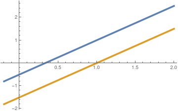
Another option to find the solution is to plot each equation and determine the intersection (if any). Mathematica helps
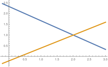
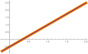
Since every linear equation in two unknowns x and y
Plot[{3*x/2 - 1/2, 3*x/2 - 1/2}, {x, -0.2, 2}, PlotStyle -> {{Thickness[0.03], Orange}, {Thickness[0.005], Blue}}]
|
|
A linear equation in the variables x₁, x₂, … , xn is an equation of the form
Observe that a linear equation does not involve products or roots of variable or any nonlinear function of these
variables. All variables occur only to the first power and do not appear as their products.
In general, we claim that a linear system of two equations with two unknowns either has a unique solution, or no solution, or infinitely many solutions.
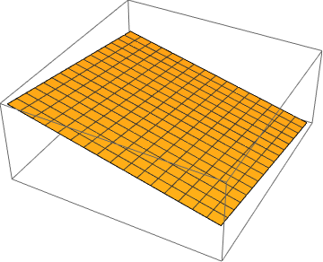
Now we turn our attention to three linear equations in three unknowns:
|
We plot one plane using the equation
\[
a\,x + b\,y + c\,z = a\,x_0 + b\,y_0 + c\, z_0 ,
\]
that passes through the point (x0, y0, z0) and having
normal vector (𝑎, b, c).
a = 3; b = 2; c = 1; x0 = -1; y0 = 1; z0 = 2;
f[x_, y_] = (a*x0 + b*y0 + c*z0 - a*x - b*y)/c; Plot3D[f[x, y], {x, -1, 1}, {y, -1, 1}, Axes -> False] |
|
|
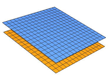
Next figure shows that there is no solution when two coincident planes parallel to the third; no common
intersection.
a = 3; b = 2; c = 1; x0 = -1; y0 = 1; z0 = 2;
f[x_, y_] = (a*x0 + b*y0 + c*z0 - a*x - b*y)/c; Plot3D[{f[x, y], 7 - (a*x + b*y)/c}, {x, -1, 1}, {y, -1, 1}, Boxed -> False, Axes -> False] |
|
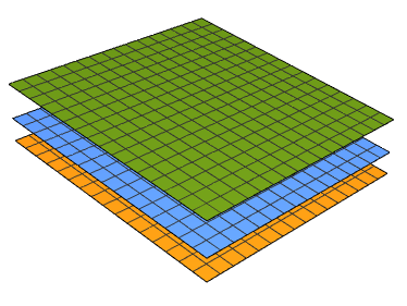
This graph shows the case of no solution because three parallel planes have no common intersection.
a = 3; b = 2; c = 1; x0 = -1; y0 = 1; z0 = 2;
f[x_, y_] = (a*x0 + b*y0 + c*z0 - a*x - b*y)/c; Plot3D[{f[x, y], 7 - (a*x + b*y)/c, 16 - (a*x + b*y)/c}, {x, -1, 1}, {y, -1, 1}, Boxed -> False, Axes -> False] |
|
|
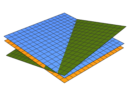
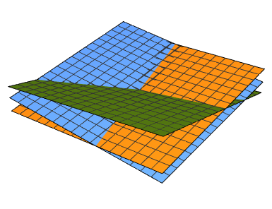
Next figure shows that there is no solution when two parallel planes crosses the third; no common
intersection.
a = 3; b = 2; c = 1; x0 = -1; y0 = 1; z0 = 2;
f[x_, y_] = (a*x0 + b*y0 + c*z0 - a*x - b*y)/c; Plot3D[{f[x, y], 7 - (a*x + b*y)/c, 5 + (12*x + 8*y)/c}, {x, -1, 1}, {y, -1, 1}, Boxed -> False, Axes -> False] |
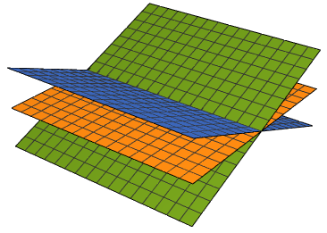
|
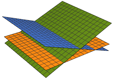
Next figure shows that there is no solution. If we substitute z = 0 (from the first equation) into
two other equations, we see that they have no common intersection.
Plot3D[{0, 10 - 10*y, 10 + 10*y}, {x, -2, 2}, {y, -2, 2},
Axes -> False, Boxed -> False]
|
|
Next figure shows that there is a unique solution. You will learn shortly how Mathematica can
detect this conclusion in a blank of eye.
Det[{{1, 2, 3}, {1, -3, 2}, {1, 4, -10}}]
Plot3D[{2*x + 3*y, -3*x + 2*y, 4*x - 10*y}, {x, -2, 2}, {y, -2, 2}, Axes -> False, Boxed -> False] |
|
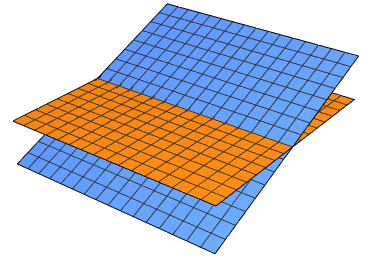
Next figure shows that there are infinitely many solutions. If we substitute z = 0 (from the first
equation) into two other equations, we see that they are equivalent.
Plot3D[{0, 10 - 10*y, 10 + 10*y}, {x, -2, 2}, {y, -2, 2},
Axes -> False, Boxed -> False]
|
|
Next figure shows that there are infinitely many solutions. If we substitute z = 0 (from the first
equation) into two other equations, we see that they are equivalent.
Plot3D[{0, 10*y}, {x, -2, 2}, {y, -2, 2}, Axes -> False,
Boxed -> False]
|
We will develop a systematic way to do this for any number of equations with arbitrary number of unknowns (often denoted as x1, x2, x3, …) through the use of matrices and vectors.
A special and important class of systems of linear equations that always have at least one solution is the class of homogeneous equations. These are systems where every bi = 0, i = 1, 2, … , m. One solution to such a system will always be when each variable is 0. This means for a system of two or three variables, the graph of each equation in a homogeneous system passes through the origin.
Matrix Notation

-
Which of the following are linear equations? If an equation is not a linear equation,
tell why.
\[ {\bf (a)} \quad 6\,x + x\,y + 3\, z = 2; \qquad {\bf (b)} \quad 5\,a -\pi + 3\,b =0; \]\[ {\bf (c)} \quad \cos \left( \frac{\pi}{2} \right) x^2 -\sin (\pi )\, x\,y + 2\, z = 6; \qquad {\bf (d)} \quad \sqrt{x} -3\,y -z =1. \]
-
Solve each system of equations.
\[ {\bf (a)} \quad \begin{cases} 2\,x + 3\,y &= 2, \\ -4\,x-y &= 1; \end{cases} \qquad {\bf (b)} \quad \begin{cases} 2\,x + 4\,y &= -4, \\ 3\,x+ 5\,y &= \phantom{-}1 . \end{cases} \]
- Find the point of intersection of the lines x −4y = −2 and 3x + 2y = 8.
-
Solve systems of equations:
\[ {\bf (a)} \quad \begin{split} \phantom{x} - 3\,y +4\,z&= \phantom{-}28, \\ 2\,x-8\,y + 6\,z &= -42 , \\ -5\,x +5\,y -2\,z &= \phantom{-}56; \end{split} \qquad {\bf (b)} \quad \begin{split} 2\,x - 2\,y + z&= 145, \\ 3\,x -y + 10\,z &= 203, \\ x+ 2\,y + 6\,z &= \phantom{1}58; \end{split} \]\[ {\bf (c)} \quad \begin{split} 2\,x - 2\,y + z &= 75, \\ \phantom{x+} 2y + 6\,z &= 30 , \\ x + 2y +2z &= 0; \end{split} \qquad {\bf (d)} \quad \begin{split} 4\,x + 5\,y -z &= 310, \\ 2x+ 3\,y + 2z &= 0, \\ 8x+ 5\,y + 4z &= 186 . \end{split} \]
-
In the study of heat transfer, it is important to determine the steady-state temperature distribution of a
thin plate when the temperature around the boundary is known (usually from an experiment or other
measurement). Let us consider the plate shown in Figure below representing a cross section of a metal beam,
with negligible heat flow in the direction perpendicular to the plate. Let t₁, t₂,
t₃, t₄ denote the temperatures at the four interior nodes of the mesh in Figure. The
temperature at a particular node is approximately equal to the average of the four nearest nodes---to the
left, above, to the right, and below.
Write a system of four equations whose solution gives estimates for the temperatures t₁, t₂, t₃, t₄.
h1 = Graphics[Line[{{0, 0}, {1.5, 0}}]];
h2 = Graphics[Line[{{0, 0.5}, {1.5, 0.5}}]];
h3 = Graphics[Line[{{0, 1}, {1.5, 1}}]];
h4 = Graphics[Line[{{0, 1.5}, {1.5, 1.5}}]];
v1 = Graphics[Line[{{0, 0}, {0, 1.5}}]];
v2 = Graphics[Line[{{0.5, 0}, {0.5, 1.5}}]];
v3 = Graphics[Line[{{1, 0}, {1, 1.5}}]]; v4 = Graphics[Line[{{1.5, 0}, {1.5, 1.5}}]];
text1 = Graphics[ Text[Style[Quantity[16, "DegreesCelsius"], FontSize -> 16], {-0.15, 0.5}]];
text2 = Graphics[ Text[Style[Quantity[18, "DegreesCelsius"], FontSize -> 16], {-0.15, 1.0}]];
text3 = Graphics[ Text[Style[Quantity[22, "DegreesCelsius"], FontSize -> 16], {0.5, -0.1}]];
text3a = Graphics[ Text[Style[Quantity[24, "DegreesCelsius"], FontSize -> 16], {0.5, 1.6}]];
text4 = Graphics[ Text[Style[Quantity[28, "DegreesCelsius"], FontSize -> 16], {1.0, -0.1}]];
text4a = Graphics[ Text[Style[Quantity[30, "DegreesCelsius"], FontSize -> 16], {1.0, 1.6}]];
text5 = Graphics[ Text[Style[Quantity[36, "DegreesCelsius"], FontSize -> 16], {1.65, 0.5}]];
text6 = Graphics[ Text[Style[Quantity[38, "DegreesCelsius"], FontSize -> 16], {1.65, 1.0}]];
t1 = Graphics[ Text[Style[Subscript[t, 1], FontSize -> 20, Purple], {0.6, 1.1}]];
t2 = Graphics[ Text[Style[Subscript[t, 2], FontSize -> 20, Purple], {1.1, 1.1}]];
t3 = Graphics[ Text[Style[Subscript[t, 3], FontSize -> 20, Purple], {1.1, 0.6}]];
t4 = Graphics[ Text[Style[Subscript[t, 4], FontSize -> 20, Purple], {0.6, 0.6}]];
d1 = Graphics[{Red, Disk[{0.5, 0.5}, 0.03]}];
d2 = Graphics[{Red, Disk[{0.5, 1.0}, 0.03]}];
d3 = Graphics[{Red, Disk[{1.0, 0.5}, 0.03]}];
d4 = Graphics[{Red, Disk[{1.0, 1.0}, 0.03]}];
Show[h1, h2, h3, h4, v1, v2, v3, v4, text1, text2, text3, text3a, text4, text4a, text5, text6, t1, t2, t3, t4, d1, d2, d3, d4]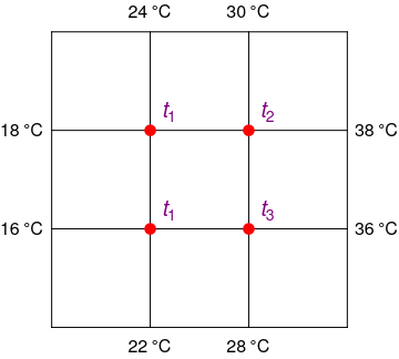
Temperature distribution -
Cubic spline interpolation provides a polynomial approximation that has smaller error than some other
interpolating polynomials such as Lagrange polynomial and Newton polynomial. Suppose you need to interpolate a
function f on some interval [x₁, x₂] given its values at end points
f₁ = f(x₁) and f₂ = f(x₂). If you know the
values of derivatives at these end points g₁ = f'(x₁) and g₂ =
f'(x₂), find a system of linear equations for coefficients of cubic polynomial
p(x) = 𝑎 x³ + b x² +
c x + d so that this polynomial matches the values of f at end points
f₁, f₂ and the values of its derivatives at end points g₁,
g₂.
Write a system of four equations for four unknowns 𝑎, b, c, and d.
- Suppose you are given a parabola y = 𝑎 x² + b x + c that passes through the points (x₁, y₁), (x₂, y₂), and (x₃, y₃). Determine an augmented matrix for the corresponding system of linear equations in unknowns 𝑎, b, and c.
- Suppose that you want to find values for 𝑎, b, and c such that the parabola y = 𝑎 x² + b x + c passes through the points (1, 2), (2, 5), and (−2, 3). Find (but do not solve) a system of linear equations whose solutions provide values for 𝑎, b, and c.
-
In each part of the problem, find a linear system in the unknowns x₁, x₂,
x₃, …, that corresponds to the given augmented matrix.
\[ {\bf (a)} \quad \left( \begin{array}{cccc|c} -1& 3 & 2 & -7 & 8 \\ \phantom{-}2 & 1 & 0 & -8 & 7 \\ \phantom{-}6 & 8 & 3 & \phantom{-}2 & 5 \end{array} \right) , \qquad {\bf (b)} \quad \left( \begin{array}{cccc|c} \phantom{-}3& -2 & 7 & -1 & 6 \\ \phantom{-}4 & -1 & 9 & -5 & 8 \\ -1 & \phantom{-}6 & 4 & \phantom{-}9 & 2 \end{array} \right) , \]\[ {\bf (c)} \quad \left( \begin{array}{cccc|c} -2& 7 & -6 & \phantom{-}2 & 7 \\ \phantom{-}5 & 2 & \phantom{-}9 & -2 & 1 \\ -4 & 4 & \phantom{-}7 & \phantom{-}5 & 3 \\ \phantom{-}2 & 4 & -5 & -1 & 2 \end{array} \right) , \qquad {\bf (d)} \quad \left( \begin{array}{cccc|c} \phantom{-}8& -3 & 5 & -6 & 1 \\ \phantom{-}2 & -7 & 5 & -4 & 2 \\ -1 & \phantom{-}4 & 2 & \phantom{-}9 & 4 \\ \phantom{-}4 & \phantom{-}7 & 9 & -2 & 3 \end{array} \right) . \]
-
In each part of the problem, find the augmented matrix for the linear system.
\[ {\bf (a)} \quad \begin{cases} \phantom{-}3\,x_2 &= \phantom{-}6, \\ -4\,x_2 &= -8 , \\ \phantom{-}5\, x_2 &= 10; \end{cases} \qquad {\bf (b)} \quad \begin{cases} 2\,x_1 + 7\,x_2 + x_3 &= -4, \\ 9\,x_2 + 2\,x_3 &= \phantom{-}1; \end{cases} \]\[ {\bf (c)} \quad \begin{cases} \phantom{-}7\,x_1 - 3\,x_2 + 3\,x_3 &= -1, \\ -4\,x_1 + 6\,x_2 - 2\,x_3 &= -2 , \\ \phantom{-}5\,x_1 + 3\, x_2 - 7\,x_3 &= \phantom{-}1; \end{cases} \qquad {\bf (d)} \quad \begin{cases} \phantom{-}x_1 - 5\,x_2 + 2\,x_3 &= -3, \\ \phantom{-}3\,x_1 - 4\,x_2 + 5\,x_3 &= \phantom{-}3, \\ -4\,x_1 - 6\,x_2 + 9\,x_3 &= -5, \end{cases} \]
- Higham, Nicholas, Gaussian Elimination, Manchester Institute for Mathematical Sciences, School of Mathematics, The University of Manchester, 2011.
- Lay, D.C., Lay, S.R., McDonald, J.J., Linear Algebra and its Applications, Pearson.