Before we dance with vector products, we remind the basic product that is not related to any vector structure. For any two sets A and B, their Cartesian product consists of all ordered pairs (𝑎, b) such that 𝑎 ∈ A and b ∈ B,
\[
A \times B = \left\{ (a,b)\,:\ a \in A, \quad b\in B \right\} .
\]
If sets A and B carry some algebraic structure, as in our case, they are vector spaces, then we can define a suitable structure on the product set as well. So, direct product is like Cartesian product, but with some additional structure. In our case, we equip it with addition operation
\[
k \left( a , b \right) = \left( k\,a , k\,b \right) , \qquad k \in \mathbb{F}.
\]
With these operations (addition and scalar multiplication) the direct product of two vector spaces becomes a vector space that is isomorphic to their direct product: V × W ≌ V ⊕ W. However, the direct product or sum is not linear in
its arguments. The tensor product V ⊗ W fixes this deficiency.
Here 𝔽 is a field of scalars (either ℚ, rational numbers, or ℝ, real numbers, or ℂ, complex numbers). It is a custom to denote the direct product of two or more scalar fields as 𝔽² or, in case of n multiples, as 𝔽n.
In 1844, Hermann Grassmann (1809--1877) published (from his own pocket) a book on geometric algebra not tied to dimension two or three. Grassmann develops several products, including a cross product represented then by brackets.
In 1877, to emphasize the fact that the result of a dot product is a scalar while the result of a cross product is a vector, William Kingdon Clifford (1845--1879) coined the alternative names scalar product and vector product for the two operations. These alternative names are still widely used in the literature.
In 1881, Josiah Willard Gibbs (1839--1903), and independently Oliver Heaviside (1850--1925), introduced the notation for both the dot product and the cross product using a period (a ⋅ b) and an "×" (a × b), respectively, to denote them.
The German physicist Woldemar Voigt (1850--1919), a student of Ernst Neumann,
used tensors for a description of stress and strain on crystals in
1898 (Die fundamentalen physikalischen Eigenschaften der Krystalle in elementarer Darstellung,
Verlag von Veit & Comp., Leipzig, 1898). Tensor
comes from the Latin tendere, which means “to stretch”.
The Italian mathematician Gregorio Ricci-Curbastro (1853--1925) and his student Tullio Levi-Civita (1873--1941) are credited for invention and popularization of tensor calculus. One of Albert Einstein's most-notable contributions to the world of mathematics is his application of tensors in general relativity theory.
Abstract mathematical formulation was done in the middle of twentieth century by Alexander Grothendieck (1928--2014).
The wedge product symbol took several years to mature from Hermann Grassmann's work (The Theory of Linear Extension, a New Branch of Mathematics, 1844) and Élie Cartan’s book on differential forms published in 1945.
The wedge symbol ∧ seems to have originated with Claude Chevalley (1909--1984) sometime between 1951 and 1954 and gained widespread use after that.
Vector Products
For high-dimensional mathematics and physics, it is important to have the right tools and symbols with which to work. This section provides an introduction for constructing a large variety of vector spaces from known spaces.
Besides direct products, we consider other versions of its generalizations.
Let V be a vector space over the field 𝔽, where 𝔽 is either ℚ (rational numbers) or ℝ (real numbers) or ℂ (complex numbers). The bilinear functions from V × V into 𝔽 were considered in sections regarding dot product and inner product.
In this section, we consider two important vector products, known as tensor product and cross product, as well as its generalization wedge product (also known as exterior product).
Our exposition is an attempt to bridge the gap between the elementary and advanced understandings of tensor product, including wedge product.
Tensor product
The tensor product is an operation combining two smaller vector spaces into one larger vector space. Elements of this larger space are called tensors.
Unfortunately, mathematicians and physicists often present tensors and the tensor product
in very different ways, sometimes making it difficult for a reader to see that
authors in different fields are talking about the same thing. This short subsection cannot embrace a diversity of tensor applications, so it follows more abstract approach, which closer related to to the linear algebra course. A section in Part 7 presents a particular application of asymmetric tensors to vector calculus and Stokes theorem.
Let V and U be two finite dimensional spaces over the same field of scalars 𝔽. Let α = { v1, v2,
… , vn } and β = { u1, u2, … , um } be their bases, respectively. Then the tensor product of vector spaces V and U, denoted by V⊗U, is spanned on the basis { vi⊗uj : i = 1, 2, … , n; j = 1, 2,… , m }. Elements of V⊗U are called tensors that are linear combinations of nm of basis vectors
\[
\sum_{i,j} \tau^{i,j} v_i \otimes u_j , \qquad \tau^{i,j} \in \mathbb{F} ,
\]
satisfying the following two (bilinear) axioms:
\begin{equation} \label{EqTensor.1}
\begin{split}
c\left( {\bf v} \otimes {\bf u} \right) = \left( c\, {\bf v} \right) \otimes {\bf u} = {\bf v} \otimes \left( c\,{\bf u} \right) , \qquad c\in \mathbb{F},
\end{split}
\end{equation}
and
\begin{equation} \label{EqTensor.2}
{\bf a} \otimes {\bf u} + {\bf b} \otimes {\bf u} = \left( {\bf a} + {\bf b} \right) \otimes {\bf u} , \\
{\bf v} \otimes {\bf u} + {\bf v} \otimes {\bf w} = {\bf v} \otimes \left( {\bf u} + {\bf w} \right) .
\end{equation}
This definition does not specify the structure of basis elements vi⊗uj, but gives a universal
mapping property involving.
Therefore, tensor product can be applied to a great variety of objects and structures, including vectors, matrices, tensors, vector spaces, algebras, topological vector spaces, and modules among others. The most familiar case is, perhaps, when A = ℝm and B = ℝn. Then, ℝm⊗ℝn ≌ ℝmn (see Example 4).
From a mathematical viewpoint it is, of course, not a good idea to introduce a new concept in a basis-dependent way. However, there is known a basis-independent
definition of V ⊗ W, as the space of bi-linear maps V* × W* ⇾ 𝔽 of the direct product of duals spaces into the scalar field. So dim(V ⊗ W) = dim(V) dim(W).
There are known two interpretations of tensor product, and both are widely used. Since the tensor product of n-dimensional vector \( \displaystyle {\bf a} = a_1 {\bf u}_1 + a_2 {\bf u}_2 + \cdots + a_n {\bf u}_n \) and m-dimensional vector \( \displaystyle {\bf b} = b_1 {\bf v}_1 + b_2 {\bf v}_2 + \cdots + b_m {\bf v}_m \) has dimension nm, it is natural to represent this product in matrix form:
Here \( \displaystyle \overline{b} = b^{\ast} = x -{\bf j}\,y \) is complex conjugate of complex number b = x + jy and j is the imaginary unit on complex plane ℂ, so j² = −1.
This approach is common, for instance, in digital image processing where images are represented by rectangular matrices. Hence, matrix representation \eqref{EqTensor.3} of the tensor product deserves a special name:
An outer product is the tensor product of two vectors \( {\bf u} = \left[ u_1 , u_2 , \ldots , u_m \right] \) and
\( {\bf v} = \left[ v_1 , v_2 , \ldots , v_n \right] , \) denoted by \( {\bf u} \otimes {\bf v} , \) is
an m-by-n matrix W such that its coordinates satisfy \( w_{i,j} = u_i v_j^{\ast} . \)
The outer product \( {\bf u} \otimes {\bf v} , \) is equivalent to a matrix multiplication
\( {\bf u} \, {\bf v}^{\ast} , \) (or \( {\bf u} \, {\bf v}^{\mathrm T} , \) if vectors are real) provided that u is represented as a
column \( m \times 1 \) vector, and v as a column \( n \times 1 \) vector. Here \( {\bf v}^{\ast} = \overline{{\bf v}^{\mathrm T}} . \)
In particular, u ⊗ v is a matrix of rank 1, which means that most matrices
cannot be written as tensor products of two vectors. The special case constitute elements ei ⊗ ej that form the matrix
which is 1 at (i, j) and 0 elsewhere, and the set of all such matrices forms a
basis for the set of m × n -matrices, denoted by ℝm,n. Note that we use the field of real numbers as an example.
On the other hand, in quantum mechanics, it is a custom to represent tensor product of two vectors as a long (column) vector of length n + m, similarly to an element from the direct product.
For example, the state of two-particle system can be described by something called a density matrix ρ on the tensor product of their respective spaces ℂn⊗ℂn. A density matrix is a generalization of a unit vector—it accounts for interactions between the two particles.
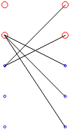
The vector representation of the tensor product itself captures all ways that basic things can "interact" with each other! We can visualize this situation in the following picture showing interactions of basis elements of the tensor product of 2- and 3-vectors.
It is possible to represent a tensor product of two vectors of length m and n as a single vector of length mn. However, this approach, known as the Kronecker product, is less efficient than vector representation embedded from the direct product. Therefore, the Kronecker product is described in matrix area where it originated.
There is a similarity between the direct product V ⊕ U and the tensor product V ⊗ U: the space V ⊕ U consists of pairs (v, u) with v∈V and u∈U, while V ⊗ U is built from vectors v⊗u. Multiplication by scalars in tensor product are defined according to the rule (axiom) in Eq.(1) and addition is formulated in Eq.\eqref{EqTensor.2}. So we see that these two operations completely different from the addition and multiplication in the direct product.
This seemingly innocuous changes clearly have huge implications on the structure of the tensor space. It can be shown that the tensor product V ⊗ U is a vector space because it is a quotient space of the product space (we wouldn’t prove it, see, for instance, Phil Lucht works).
Let us introduce the basis vectors x = (1, 0) and y = (0, 1), then
\begin{align*}
{\bf u} \otimes {\bf v} &=
(2, 1) \otimes (1, 4) + (2, -3) \otimes (-2, 3)
\\
&= \left( 2x + y \right) \otimes \left( x + 4y \right) + \left( 2x -3y \right) \otimes \left( -2x + 3y \right)
\\
&= 2 x \otimes x + 8 x \otimes y + y \otimes x + 4 y \otimes y - 4 x \otimes x + 6 x \otimes y + 6 y \otimes x - 9 y \otimes y
\\
&= - 2 x \otimes x + 14 x \otimes y + 7 y \otimes x - 5 y \otimes y .
\end{align*}
Example 4:
First, we consider a simple case of m = n, and find ℝ>⊗ℝ. It is spanned on the single basis vector i⊗j, where i and j are unit vectors on ℝ (hence, they are the same). Hence, ℝ⊗ℝ can be visualized by the line (x, x) drawn on the plane ℝ².
In general, we have ℝm,1⊗ℝ1,n ≌ ℝm,n with the product
defined to be u⊗v = uv, the matrix product of a column and a row vector. Of course, these two spaces 𝔽m,n and 𝔽n,m are naturally isomorphic to each other, 𝔽m,n ≌ 𝔽n,m, so in that
sense they are the same, but we would never write v ⊗ u when we mean u ⊗ v.
Outer[Times, {1 + I, 2, -1 - 2*I, 2 - I} ,
Conjugate[{3 + I, -1 + I, 2 - I}]]
{{1 + I}, {2}, {-1 - 2*I}, {
2 - I}} .Conjugate[{{3 + I, -1 + I, 2 - I}}]
{{4 + 2 I, -2 I, 1 + 3 I}, {6 - 2 I, -2 - 2 I,
4 + 2 I}, {-5 - 5 I, -1 + 3 I, -5 I}, {5 - 5 I, -3 - I, 5}}
MatrixRank[%]
Out[3]= 1
which is rank 1 matrix.
End of Example 5
■
Example 6:
Let V = 𝔽[x] be
vector space of polynomials in one variable. Then V ⊗ V =
𝔽[x₁, x₂] is the space of polynomials in two variables, the product is defined to be p(x)⊗q(x) = p(x₁) q(x₂).
Note: this is not a commutative product, because in general
\[
p(x)\otimes q(x) = p\left( x_1 \right) q\left( x_2 \right) \ne q \left( x_1 \right) p \left( x_2 \right) = q\left( x \right) \otimes p \left( x \right) .
\]
End of Example 6
■
Example 7:
If V is any vector space over 𝔽, then V ⊗ 𝔽 ≌ V. In this case, tensor product, ⊗, is just
scalar multiplication.
End of Example 7
■
Example 8:
If V and U are finite dimensional vector spaces over field 𝔽, then V* = ℒ(V, 𝔽) is the set of all linear functionals on V. Hence, V* ⊗ U = ℒ(V, U), with multiplication defined as φ⊗u ∈ ℒ(V, U) is the linear transformation from V to U because (φ⊗u)(v) = φ(v)⋅u, for φ ∈ V* and u ∈ U.
This result is just the abstract version of Example 4. If V = 𝔽n,1 and U = 𝔽m,1, then V* = 𝔽1,n. From Example 4, V ⊗ U is identified with 𝔽m,n, which is in turn identified
with ℒ(V, U), the set of all linear transformations from V to U.
Note: If V and U are both infinite dimensional, then V* ⊗ U is a subspace of ℒ(V, U), but not equal to it because linear combinations include only finite number of terms. Specifically, V* ⊗ U = { T ∈ ℒ(V, U) : dim range(T) < ∞ } is the set of finite rank linear transformations in ℒ(V, U), the space of all linear functions from V to U. Recall that the tensor product V* ⊗ U consists of only finite number of linear combinations of rank 1 elements φ⊗u.
End of Example 8
■
Example 9:
Let us consider ℚn and ℝ as vector spaces over the field of rational numbers. Then ℚn⊗ℝ is isomorphic as a vector space over ℚ to ℝn, where the multiplication is just scalar multiplication on ℝn.
Let α = { e1, e2, … , en } be the standard basis for ℚn and let β be an infinite basis for ℝ over ℚ. First we show that α⊗β spans ℝn. Let (𝑎1, 𝑎2, … , 𝑎n) ∈ ℝn. Every component can be expanded into finite sum
\( \displaystyle a_i = \sum_j b_{ij} x_j , \quad i=1,2,\ldots , n , \) where xi ∈ β. Thus,
\( \displaystyle ( a_1 , a_2 , \ldots , a_n ) = \sum_{ij} b_{ij} {\bf e}_i \otimes x_j . \)
Next we show that α⊗β is linearly independent. Suppose opposite \( \displaystyle \sum_{i,j} c_{ij} {\bf e}_i \otimes x_j = 0 . \) Since
\[
\sum_{i,j} c_{ij} {\bf e}_i \otimes x_j = \left( \sum_j c_{1,j} x_j , \sum_j c_{2,j} x_j , \ldots , \sum_j c_{n,j} x_j , \right) ,
\]
we have \( \displaystyle \sum_{j} c_{ij} x_j = 0 , \) for all i. Since { xi } are linearly independent, cij = 0, as required.
End of Example 9
■
Vector or Cross product
It is well-known that a vector space can be equipped with a product operation (besides vector addition) only for dimensions 1 and 2. The cross product is a successful attempt to implement the product in a three-dimensional vector space, but loosing commutative property of multiplication. On the other hand, the outer product assigns a matrix to two vectors of arbitrary size.
For any two vectors in ℝ³, \( \displaystyle {\bf a} = \left[ a_1 , a_2 , a_3 \right] \) and \( \displaystyle {\bf b} = \left[ b_1 , b_2 , b_3 \right] , \) their
cross product is the vector
Here \( \displaystyle \hat{\bf e}_1 , \ \hat{\bf e}_2 , \ \hat{\bf e}_3 \ \) are unit vectors in ℝ³ that are also usually denoted by i, j, and k, respectively.
Cross product of two vectors a and b from ℝ³ can be defined by
θ is the angle between a and b in the plane containing them (hence, it is between 0 and π);
∥ x ∥ is the Euclidean norm, so \( \displaystyle \| {\bf x} \| = \| (x_1 , x_2 , x_3 )\| = \sqrt{x_1^2 + x_2^2 + x_3^2} ; \)
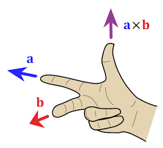
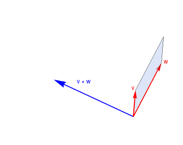
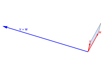
n is a unit vector perpendicular to the plane containing a and b, with direction such that the ordered set (a, b, n) is positively-oriented. Conventionally, direction of n is given by the right-hand rule, where one simply points the forefinger of the right hand in the direction of a and the middle finger in the direction of b. Then, the vector n is coming out of the thumb (see the adjacent picture).
Right hand rule.
Cross product.
We plot with Mathematica cross product of two vectors using DynamicModule command so you can see the value of cross product, which is the area of parallelogram formed by two given vectors---it is marked in blue.
The cross product is indeed perpendicular to the original vectors
VectorAngle[v, k]/Degree
VectorAngle[w, k]/Degree
90
End of Example 10
■
Despite that the cross product is identified uniquely by three entries, there is something very peculiar about the vector u × v. If u and v are orthogonal unit vectors, then the vectors u, v, u × v form a right-handed coordinate system. But if R ∈ ℝ³ is the linear transformation that mirrors vectors in the u, v plane, then { Ru, Rv, R(u×v) } = { u, v, −u×v } forms a left-handed coordinate system. In general, the cross product obeys the following identity under matrix transformation:
where M is a 3×3 matrix and M−T is the transpose of the inverse matrix.
Thus, u×v does not really transform as a vector. This anomaly should alert us to the fact that cross product is not really a true vector. In fact, cross product transforms more like a tensor than a vector.
(−u) × (−v)
Cross product of negative vectors
Example 11:
Let us consider two vectors a = [ 2, −1, −1 ] and b = [ −1, 2, 1 ]. Their cross product is
ab = {1, -1, 3};
sM = Transpose[Inverse[M]] ;
sM.ab
{7, 16, -26}
End of Example 11
■
One of the main motivations to use cross product comes from classical mechanics: A torque τ about a point due to a force F
acting at another point at distance r is expressed through cross product: τ = r × F.
\begin{equation} \label{EqCross.4}
\varepsilon_{i,j,k} = \begin{cases}
\phantom{-}0 , & \quad\mbox{if any two labels are the same},
\\
-1, & \quad \mbox{if }i,\, j,\,k \mbox{ is an odd permutation of 1, 2, 3}, \\
\phantom{-}1 , & \quad \mbox{if } i,\, j,\,k \mbox{ is an even permutation of 1, 2, 3}.
\end{cases}
\end{equation}
The Levi-Civita symbol εijk is a tensor of rank three and is anti-symmetric on each pair of indexes.
The determinant of a matrix A with elements 𝑎ij can be written in term of εijk
Given two space vectors, a and b, we can find a third space vector c, called
the cross product of a and b, and denoted by c = a × b. The magnitude
of c is defined by |c| = |a| |b| sin(θ), where θ is the angle between a and b.
The direction of c is given by the right-hand rule: If a is turned to b (note the order in which a and b appear here) through the angle between a and b, a (right-handed) screw that is perpendicular to a and b will advance in the
direction of a × b. This definition implies that
Using these properties, we can write the vector product of two vectors in terms
of their components. We are interested in a more general result valid in other
coordinate systems as well. So, rather than using x, y, and z as subscripts for
unit vectors, we use the numbers 1, 2, and 3. In that case, our results can
also be used for spherical and cylindrical coordinates which we shall discuss
shortly.
Actually, there does not exist a cross product vector in space with more than 3 dimensions.
The fact that the cross product of 3 dimensions vector gives an object which also has 3 dimensions
is just pure coincidence.
Theorem 2:
The cross product in 3 dimensions is actually a tensor of rank 2 with 3 independent coordinates.
Example 13:
From the definition of the vector product, it follows that
\[
\left\vert {\bf a} \times {\bf b} \right\vert = \mbox{ area of the parallelogram defined by} \quad {\bf a} \mbox{ and } {\bf b} .
\]
So we can use Eq.\eqref{EqCross.6} to find the area of a parallelogram defined by two
vectors directly in terms of their components. For instance, the area defined by
a = (1, −1, 2) and b = (−2, 3, 1) can be found by calculating their vector product
Example 14:
The volume of a parallelepiped defined by three non-coplanar vectors a, b, and c is given by \( \displaystyle \left\vert {\bf a} \cdot \left( {\bf b} \times {\bf c} \right) \right\vert . \) The absolute value is taken to ensure the positivity of the area. In terms of components we have
Coordinates are “functions” that specify points of a space. The smallest
number of these functions necessary to specify a point P is called the dimension of that space.
There are
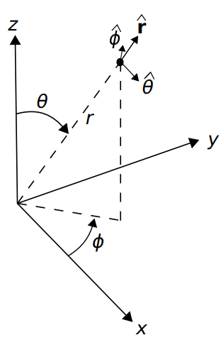
three widely used coordinate systems in a three-dimensional vector space ℝ³: Cartesian (x(P), y(P), z(P)), cylindrical (ρ(P), φ(P), z(P)), and spherical (r(P), θ(P), φ(P)). The latter φ(P) is called
the azimuth or the azimuthal angle of P, while θ(P) is called its polar angle.
Spherical coordinates
For r > 0, 0 < θ ≤ π, 0 ≤ φ ≤ 2π, we have spherical coordinates
\[
\begin{split}
x &= r\,\sin\theta \,\cos\varphi , \\
y &= r\,\sin\theta \,\sin\varphi , \\ %\qquad
z &= r\,\cos\theta , \end{split}
\]
where
\[
r = \sqrt{x^2 + y^2 + z^2},
\]
and
\[
\theta = \arccos \frac{z}{r} = \begin{cases}
\mbox{indeterminate} , & \quad \mbox{ if } x=0 \ \mbox{ and }\ y = 0, \ \mbox{ and }\ z = 0,
\\
\arctan \frac{\sqrt{x^2 + y^2}}{z} , & \quad \mbox{ if } \ z > 0,
\\
\pi + \arctan \frac{\sqrt{x^2 + y^2}}{z} , & \quad \mbox{ if } \ z < 0,
\\
+ \frac{\pi}{2} , & \quad \mbox{ if } z = 0 \ \mbox{ and }\ y \ne 0,
\end{cases}
\]
\[
\varphi = \mbox{sign}(y)\,\arccos \frac{x}{\sqrt{x^2 + y^2}} = \begin{cases}
\mbox{indeterminate} , & \quad \mbox{ if } x=0 \ \mbox{ and }\ y = 0,
\\
\arctan \left( \frac{y}{x} \right) + \pi , & \quad \mbox{ if } x > 0,
\\
\arctan \left( \frac{y}{x} \right) + \pi , & \quad \mbox{ if } x < 0, \ \mbox{ and }\ y \ge 0,
\\
\arctan \left( \frac{y}{x} \right) - \pi , & \quad \mbox{ if } x < 0, \ \mbox{ and }\ y < 0,
\\
+ \frac{\pi}{2} , & \quad \mbox{ if } x = 0 \ \mbox{ and }\ y > 0,
\\
- \frac{\pi}{2} , & \quad \mbox{ if } x = 0 \ \mbox{ and }\ y < 0.
\end{cases}
\]
Mathematica has three multiplication commands for vectors: the dot (or inner) and outer products (for arbitrary vectors), and
the cross product (for three dimensional vectors).
The cross product can be done on two vectors. It is important to note that the cross product is an operation that is only functional in three dimensions. The operation can be computed using the Cross[vector 1, vector 2] operation or by generating a cross product operator between two vectors by pressing [Esc] cross [Esc]. ([Esc] refers to the escape button)
Cross[{1,2,7}, {3,4,5}]
{-18,16,-2}
Example 17:
Let us consider a rigid body which rotates around the origin O. To avoid having to carry out integrals, we will think of the rigid body as consisting of (a possibly large number of) mass points, labeled by an index α, each with mass mα, position vector rα and velocity vα. The total kinetic energy of this body is of course obtained by summing over the kinetic energy of all mass points, that is
\( \displaystyle E = \frac{1}{2} \sum_{\alpha} m_{\alpha} {\bf v}_{\alpha}^2 . \)
Since the body is rigid, the velocities of the mass points are not independent but are related to their positions by vα = ω × rα, where ω is the angular velocity of the body. (The length
|ω| is the angular speed and the direction of ω indicates the axis of rotation.) The kinetic
energy of the rotating body can then be written as
The object in the square bracket, denoted by Iij, is called the moment of inertia tensor, a
characteristic quantity of the rigid body. It plays a role in rotational motion analogous to
that of regular mass in linear motion. In terms of the moment of inertia tensor, the total
kinetic energy of the rigid body can be written as
\[
E = \frac{1}{2}\,I_{ij} \omega_i \omega_j .
\]
This relation is of fundamental importance for the mechanics of rigid bodies, in particular
the motion of tops. (For more on the mechanics of rigid bodies.
Wedge or Exterior product
The wedge product of two vectors u and v measures the noncommutativity of their tensor product.
An wedge product (also known as exterior product) is the tensor product of two vectors \( {\bf u} = \left[ u_1 , u_2 , \ldots , u_n \right] \) and
\( {\bf v} = \left[ v_1 , v_2 , \ldots , v_n \right] , \) denoted u ∧ v, is the square matrix defined by
\[
{\bf v} \wedge {\bf u} = {\bf v} \otimes {\bf u} - {\bf u} \otimes {\bf v} .
\]
Equivalently,
\[
\left( {\bf v} \wedge {\bf u} \right)_{ij} = \left( v_i u_j - v_j u_i \right) .
\]
Example 18:
We are going to show that the wedge product u ∧ v has, up to sign, six, not four, distinct entries. Let u = [ 𝑎, b, c, d ] and v = [ α, β, γ, δ ] be any two vectors in ℝ4. Their wedge product is the square matrix:
\[
{\bf u} \wedge {\bf v} = \begin{bmatrix} 0 & a\beta - \alpha b & a\gamma - \alpha c & a\delta - \alpha d \\
b \alpha - \beta a & 0 & b \gamma - \beta c & b \delta - \beta d \\
c \alpha - \gamma a & c \beta - \gamma b & 0 & c \delta - \gamma d \\
d \alpha - \delta a & d \beta - \delta b & d \gamma - \delta c & 0
\end{bmatrix} .
\]
Let us introduce six parameters:
\[
c_1 = a\beta - \alpha b , \quad c_2 = a\gamma - \alpha c , \quad c_3 = a\delta - \alpha d ,
\]
and
\[
c_4 = b \gamma - \beta c , \quad c_5 = b \delta - \beta d , \quad c_6 = c \delta - \gamma d .
\]
Then the wedge product of these two vectors becomes
It can be shown that in n dimensions, the antisymmetric matrix u ∧ v has n(n − 1)/2 unique entries.
The wedge product is an antisymmetric 2-tensor, in any dimension.
Like the tensor product, the wedge product is defined for two vectors of arbitrary dimension. Notice, too, that the wedge product shares many properties with the cross product. For example, it is easy to verify directly from the definition of the wedge product as the difference of two tensor products obeys the following properties:
The wedge product also shares some other important properties with the cross product. The defining characteristics of the cross product are captured by the formulas
Moreover, in three dimensions, the entries of the wedge product matrix u ∧ v are, up to sign, the same as the components of the cross product vector u × v.
An outer product is the tensor product of two coordinate vectors \( {\bf u} = \left[ u_1 , u_2 , \ldots , u_m \right] \) and
\( {\bf v} = \left[ v_1 , v_2 , \ldots , v_n \right] , \) denoted \( {\bf u} \otimes {\bf v} , \) is
an m-by-n matrix W of rank 1 such that its coordinates satisfy \( w_{i,j} = u_i v_j . \)
The outer product \( {\bf u} \otimes {\bf v} , \) is equivalent to a matrix multiplication
\( {\bf u} \, {\bf v}^{\ast} , \) (or \( {\bf u} \, {\bf v}^{\mathrm T} , \) if vectors are real) provided that u is represented as a
column \( m \times 1 \) vector, and v as a column \( n \times 1 \) vector. Here \( {\bf v}^{\ast} = \overline{{\bf v}^{\mathrm T}} . \)
Example 19:
Let
&omega1 = 3xdx − 5ydy
and
&omega2 = 2zdx + 4xdz
Given two vectors a and b from ℝ³, find a third (non-zero!) vector v perpendicular to the first two vectors. In other words, find v such that annihilates two dot products: v
· a = 0 and v · b = 0.
Find the cross product of the following pairs of vectors.
[3, −1, 2] and [4, 2, −3];
[−3, 6, 5] and [2, −4, 1].
Two vectors u and v are separated by an angle of π/6, and |u|=3/2 and |v|=2/3. Find |u×v|.
Two vectors u and v are separated by an angle of π/4, and |u|=4 and |v|=5. Find |u×v|.
Define the triple product of three vectors, x, y, and z, to be the scalar x⋅(y×z). Show that three vectors lie in the same plane if and only if their triple product is zero. Verify that ⟨1,1,−3⟩, ⟨2,3,4⟩ and ⟨4,5,−2⟩ are coplanar.
Find the area of the parallelogram with vertices (0,0), (2,1), (7,4), and (2,3).
Find the area of the triangle with vertices (1,0,0), (3,7,4), and (−2,−3,1).
Find and explain the value of (i×j)×k and (i+j)×(i−j).
Banchoff, T.F., Lovett, S., Differential Geometry of Curves and Surfaces, Third edition, CRC Press, Boca Raton, FL, 2023.