
Markov Chains
In a probabilistic description of an experiment or process, the outcome or result is uncertain and may take any value from known set of states. For example, if a coin is tossed successively, the outcome in the n-th toss could be a head or a tail; or if an ordinary die is rolled, the outcome may be 1, 2, 3, 4, 5, or 6. Associated with each ourcome is a number p (\( 0 \le p \le 1 \) ), called the probability of the outcome, which is a measure of the likelihood of occurence of the outcome. If we denote the outcome of a roll of a die by X, then we write \( \Pr [X=i] = p_i \) to mean that the probability that X takes the value i is equal to pi, where \( p_1 + p_2 + \cdots + p_6 = 1 . \) The symbol X is called a random variable and, in general, X may take a real value.
Often we are given the information that a particular event A has occurred, in which case the probability of occurrence of another event B will be effected. This gives rise to the concept of the conditional probability of the event A given that B has occurred, which is denoted by \( \Pr [A\,|\,B] \) and defined as
Stochastic process is a process in which changing of the system from one state to another is not predetermined but can only be specified in terms of certain probabilities which are obtained from the past behavior or history of the system.
Now we are going to define a first-order Markov process or a Markov Chain as stochastic process where in the transition probability of a state depends exclusively on its immediately preceding state. A more explicit definition can be given as follows.- The outcome of the n-th trial depends only on the outcome of the (n−1)-th trial and not on the outcome of the earlier trials; and
- In two successive trials of the experiment, the probability of going from state Si to state Sj remains the same or does not change.
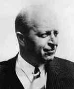
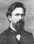
A Markov process is named after the Russian mathematician Andrey Andreyevich Markov (1856--1922), a student of Pafnuty Chebyshev (Saint Petersburg, Russia). Markov studied Markov processes in the early 20th century, publishing his first paper on the topic in 1906. Markov and his younger brother Vladimir Andreevich Markov (1871--1897) proved Markov brothers' inequality. His son, another Andrei Andreevich Markov (1903--1979), was also a notable mathematician, making contributions to constructive mathematics and recursive function theory. One of his famous Ph.D. students was Jacob/Yakov Davidovich Tamarkin (1888--1945), who upon immigration to the USA, worked since 1927 at Brown University.
Markov chains have many applications as statistical models of real-world processes, such as studying cruise control systems in motor vehicles, queues or lines of customers arriving at an airport, exchange rates of currencies, storage systems such as dams, and population growths of certain animal species. The algorithm known as PageRank, which was originally proposed for the internet search engine Google, is based on a Markov process. Furthermore, Markov processes are the basis for general stochastic simulation methods known as Gibbs sampling and Markov Chain Monte Carlo, are used for simulating random objects with specific probability distributions, and have found extensive application in Bayesian statistics.
To understand a system described by a Markov process or a Markov chain the following concepts are necessary.
If T is a regular probability matrix, then there exists a unique probability vector t such that \[ {\bf T}\,{\bf t} = {\bf t} . \] This unique probability vector is also called as a steady state vector.
Example 1: Suppose that m moleculas are distributed between urns (I) and (II), and at each step or trial, a molecule is chosen at random and transferred from its urn to the otehr urn. Let Xn denote the number of molecules in urn (I) just after the n-th step. Then \( X_0 , X_1 , \ldots \) is a Markov chain with state space \( \left\{ 0, 1, \ldots , m \right\} \) and transition probabilities are
Example 2: In \( \mathbb{R}^n , \) the vectors \( e_1 [1,0,0,\ldots , 0] , \quad e_2 =[0,1,0,\ldots , 0], \quad \ldots , e_n =[0,0,\ldots , 0,1] \) form a basis for n-dimensional real space, and it is called the standard basis. Its dimension is n.
Example 3: In state elections, it has been determined that voters will switch votes according to the following probabilities.
| Socialist | Capitalist | Independent | |
| Socialist | 0.7 | 0.35 | 0.4 |
| Capitalist | 0.2 | 0.6 | 0.3 |
| Independent | 0.1 | 0.05 | 0.3 |
The transition matrix for the Markov chain is
Theorem: Let V be a vector space and \( \beta = \left\{ {\bf u}_1 , {\bf u}_2 , \ldots , {\bf u}_n \right\} \) be a subset of V. Then β is a basis for V if and only if each vector v in V can be uniquely decomposed into a linear combination of vectors in β, that is, can be uniquely expressed in the form
If the vectors \( \left\{ {\bf u}_1 , {\bf u}_2 , \ldots , {\bf u}_n \right\} \) form a basis for a vector space V, then every vector in V can be uniquely expressed in the form
Theorem: Let S be a linearly independent subset of a vector space V, and let v be an element of V that is not in S. Then \( S \cup \{ {\bf v} \} \) is linearly dependent if and only if v belongs to the span of the set S.
Theorem: If a vector space V is generated by a finite set S, then some subset of S is a basis for V ■
A vector space is called finite-dimensional if it has a basis consisting of a finite
number of elements. The unique number of elements in each basis for V is called
the dimension of V and is denoted by dim(V). A vector space that is not finite-
dimensional is called
infinite-dimensional.
The next example demonstrates how Mathematica can determine the basis or set of linearly independent vectors from the given set. Note that basis is not unique and even changing the order of vectors, a software can provide you another set of linearly independent vectors.
MatrixRank[m =
{{1, 2, 0, -3, 1, 0},
 {1, 2, 2, -3, 1, 2},
 {1, 2, 1, -3, 1, 1},
 {3, 6, 1, -9, 4, 3}}]
Then each of the following scripts determine a subset of linearly independent vectors:
m[[ Flatten[ Position[#, Except[0, _?NumericQ], 1, 1]& /@

    Last @ QRDecomposition @ Transpose @ m ] ]]
or, using subroutine
MinimalSublist[x_List] :=

 Module[{tm, ntm, ytm, mm = x}, {tm = RowReduce[mm] // Transpose,

   ntm = MapIndexed[{#1, #2, Total[#1]} &, tm, {1}],

   ytm = Cases[ntm, {___, ___, d_ /; d == 1}]};

  Cases[ytm, {b_, {a_}, c_} :> mm[[All, a]]] // Transpose]
we apply it to our set of vectors.
m1 = {{1, 2, 0, -3, 1, 0}, {1, 2, 1, -3, 1, 2}, {1, 2, 0, -3, 2,
    1}, {3, 6, 1, -9, 4, 3}};

MinimalSublist[m1]
{{1, 1, 1, 3}, {0, 1, 0, 1}, {1, 1, 2, 4}}
One can use also the standard Mathematica command: IndependenceTest.
■
- Using matrix \( {\bf N} = \begin{bmatrix} 8 & -1 \\ 13 & 18 \end{bmatrix} , \) send message