
Introduction to Linear Algebra
Systems of Linear Equations
- Introduction
- Linear systems
- Vectors
- Linear combinations
- Matrices
- Planes in ℝ³
- Reduced Row-Echelon Form
- Equation A x = b
- Sensitivity of solutions
- Linear independence
- Plane transformations
- Space transformations
- Linear transformations
- Affine maps
- Exercises
- Answers
Matrix Algebra
- Introduction
- Manipulation of matrices
- Partitioned matrices
- Block matrices Matrix operators
- Determinants
- Cofactors
- Cramer's rule
- Equivalent matrices
- Elimination: A = L U
- PLU factorization
- Reflection
- Givens rotation
- Special matrices
- Exercises
- Answers
Vector Spaces
- Introduction
- Motivation
- Vector spaces
- Bases
- Dimension
- Coordinate systems
- Change of basis
- Linear transformations
- Matrix transformations
- Compositions
- Isomorphisms
- Dual transformations
- Direct sums
- Quotient spaces
- Rank
- Solving A x = b
- Exercises
- Answers
Eigenvalues, Eigenvectors
- Introduction
- Characteristic polynomials
- Companion matrix
- Algebraic and geometric multiplicities
- Minimal polynomials
- Eigenspaces
- Where are eigenvalues?
- Eigenvalues of A B and B A
- Generalized eigenvectors
- Similarity
- Diagonalizability
- Self-adjoint operators
Euclidean Spaces
- Introduction
- Dot product
- Bilinear transformations
- Inner product
- Norm and distance
- Matrix norms
- Dual norms
- Dual transformations
- Examples of transformations
- Orthogonality
- Gram--Schmidt Process
- Orthogonal sets
- Self-adjoint Matrices
- Unitary matrices
- Projection operators
- QR-decomposition
- Least Square Approximation
- Quadratic forms
- Exercises
- Answers
Matrix Decompositions
- Introduction
- Symmetric matrices
- LU-decomposition
- QR-decomposition
- Cholesky decomposition
- Schur decomposition
- Positive matrices
- Roots
- Polar factorization
- Spectral decomposition
- Singular values
- SVD <
- Pseudoinverse
- Exercises
- Answers
Applications
- GPS problem
- Poisson equation
- Graph theory
- Error correcting codes
- Electric circuits
- Markov chains
- Cryptography
- Wave-length transfer matrix
- Computer graphics
- Linear Programming
- Hill's determinant
- Fibonacci matrices
- Discrete dynamic systems
- Discrete Fourier transform
- Fast Fourier transform
- Curve fitting
Functions of Matrices
- Introduction
- Diagonalization
- Sylvester formula
- The Resolvent method
- Polynomial interpolation
- Positive matrices
- Roots <
- Pseudoinverse
- Exercises
- Answers
Miscellany
- Circles along curves
- TNB frames
- Tensors
- Tensors in ℝ³
- Tensors & Mechanics
- Differential forms
- Calculus
- Vector representations
- Matrix representations
- Change of basis
- Orthonormal Diagonalization
- Generalized inverse
- Differential forms
Preliminaries
- Complex Number Operations
- Sets
- Polynomials
- Polynomials and Matrices
- Computer solves Systems of Linear Equations
- Location of Eigenvalues
- Power Method
- Iterative Method
- Similarity and Diagonalization
Glossary
Reference

This Book is licensed under Creative Commons Attribution-NonCommercial-NoDerivs 3.0 Unported License
Linear Independence
Before introducing the property of independence, we remind, for convenience, the following definition.VectorQ[v1]
True
% // MatrixForm
|
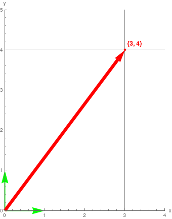
eg1 = Graphics[{Green, Thick, Arrowheads -> .08,
Arrow[{{0, 0}, basisM[[1]]}], Arrow[{{0, 0}, basisM[[2]]}],
Thickness[.02], Red, Arrow[{{0, 0}, v1}], Red,
PointSize -> Medium, Point[v1]}, Axes -> True,
PlotRange -> {{0, 4}, {0, 5}}, AxesLabel -> {"x", "y"},
GridLines -> {{v1[[1]]}, {v1[[2]]}},
Epilog -> {Red,
Text[Style[ToString[v1], FontSize -> 12, Bold], {3.25, 4.15}]}];
Labeled[eg1, "Vector {3,4}"]
|
|
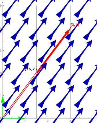
v2 = .5 v1
vp1 = VectorPlot[v1, {x, 0, 4}, {y, 0, 5}, VectorPoints -> 6, VectorMarkers -> "Dart", VectorSizes -> 1.5]; colinear1 = Graphics[{Thickness[.008], White, Arrow[{{0, 0}, v2}], PointSize -> Medium, Point[{1.5, 2}]}]; Show[eg1, vp1, colinear1, GridLines -> {{v1[[1]], 1.5}, {v1[[2]], 2}}, Epilog -> {Text[ Style[ToString[v2], FontSize -> 12, Bold], {1.25, 2.17}], Red, Text[Style[ToString[v1], FontSize -> 12, Bold], {3.20, 4.14}]}]; Labeled[%, "Equivalent Vectors"] |
% // N
{0.5, 0.866025}
|
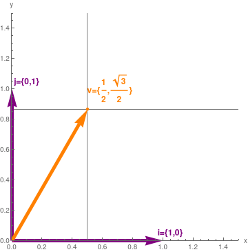
v = {1/2, Sqrt[3]/2}; Null
basisM = IdentityMatrix[2]; Null eg2 = Graphics[{Hue[5/6, 1, 1/2], Thickness[0.015], Arrowheads -> 0.08, Arrow[{{0, 0}, Part[basisM, 1]}], Arrow[{{0, 0}, Part[basisM, 2]}], Thickness[0.015], Orange, Arrow[{{0, 0}, v}], Orange, PointSize -> Medium, Point[v]}, Axes -> True, PlotRange -> {{0, 1.5}, {0, 1.5}}, AxesLabel -> {"x", "y"}, GridLines -> {{Part[v, 1]}, {Part[v, 2]}}, Epilog -> {Hue[5/6, 1, 1/2], Text[Style["i={1,0}", FontSize -> 12, Bold], {1.05, 0.05}], Hue[5/6, 1, 1/2], Text[Style["j={0,1}", FontSize -> 12, Bold], {0.1, 1.05}], Orange, Text[Style[ "v={\!\(\*FractionBox[\(1\), \ \(2\)]\),\!\(\*FractionBox[SqrtBox[\(3\)], \(2\)]\)}", FontSize -> 12, Bold], {0.65, 1}]}]; Null Labeled[eg2, "Vector {\!\(\*FractionBox[\(1\), \ \(2\)]\),\!\(\*FractionBox[SqrtBox[\(3\)], \(2\)]\)}"] |
Whereas expansion (1.1) shows the only way to express the vector (3, 4) as a linear combination of i = (1, 0) and j = (0, 1), there are infinitely many ways to express this vector (3, 4) as a linear combination of three vectors: i, j, and v. Three possibilities are shown below
3 i + 4 j + 0 v
2 i + (4 - Sqrt[3]) j + 2 v
(3 - 2 Sqrt[3]) i + 4 Sqrt[3] v - 2 j
- S is a linearly independent subset of V if and only if no vector in S can be expressed as a linear combination of the other vectors in S.
- S is a linearly dependent subset of V if and only if some vector v in S can be expressed as a linear combination of the other vectors in S.
Conversely, suppose that we have two distinct representations as linear combinations for some vector:
Mathematica confirms
mat = m.{a1, a2, a3, a4};
MatrixForm[mat]
m.sol1 == {0, 0, 0, 0}
A set of vectors is linearly independent if the only
representations of 0 as a linear combination of its vectors is the
trivial representation in which all the scalars ai are zero.
The alternate definition, that a set of vectors is linearly dependent if and
only if some vector in that set can be written as a linear combination of the
other vectors, is only useful when the set contains two or more vectors. Two
vectors are linearly dependent if and only if one of them is a constant
multiple of another.
To illustrate in ℝ³, consider the standard unit vectors that are usually labeled as
MatrixForm[%]
Conversely, if for some i, vi can be expressed as a linear combination of other elements from S, i.e., \( \displaystyle {\bf v}_i = \sum_{j\ne i} \alpha_j {\bf v}_j , \) where αj ∈ 𝔽, then this yields that \[ \alpha_1 {\bf v}_1 + \alpha_2 {\bf v}_2 + \cdots + (-1)\,{\bf v}_i + \alpha_{i+1} {\bf v}_{i+1} + \cdots + \alpha_n {\bf v}_n = 0 . \] This shows that there exist scalars α1, α2, … , αn with αi = −1 such that \( \displaystyle \sum_i \alpha_i {\bf v}_i = {\bf 0} , \) and hence S is linearly dependent.
We want to know whether or not there exist complex numbers c₁, c₂, and c₃, such that the identity matrix I = σ0 is a linear combination of the Pauli matrices: \[ {\bf I} = \sigma_0 = c_1 \sigma_1 + c_2 \sigma_2 + c_3 \sigma_3 . \] Writing this equation more explicitly gives \[ \begin{bmatrix} 1 & 0 \\ 0 & 1 \end{bmatrix} = c_1 \begin{bmatrix} 0 & 1 \\ 1 & 0 \end{bmatrix} + c_2 \begin{bmatrix} 0 & -{\bf j} \\ {\bf j} & \phantom{-}0 \end{bmatrix} + c_3 \begin{bmatrix} 1 & \phantom{-}0 \\ 0 & -1 \end{bmatrix} \] This is equivalent to four linear equations: \begin{align*} 1 & = c_3 \\ 0 &= c_1 - {\bf j}\,c_2 , \\ 0 &= c_1 + {\bf j}\,c_2 , \\ 1 &= - c_3 \end{align*} Since c₃ cannot be equal 1 and −1 simultaneously, we conclude that this system of equations has no solution and this set of Pauli matrices together with the identity matrix is linearly independent.
Mathematica confirms
eqns = c1 {{0, 1}, {1, 0}} + c2 {{0, -j}, {j, 0}} + c3 {{1, 0}, {0, -1}};
Grid[{{MatrixForm[IdentityMatrix[2]], "=", MatrixForm[eqns]}}] Grid[{{Column[Flatten[IdentityMatrix[2]]], Column[{"=", "=", "=", "="}], Column[Flatten[eqns]]}}]
0 = c1 - c2 j
0 = c1 - c2 j
1 = c3
A set containing a single vector {v}, where v ∈ V, is linearly independent if and only if v ≠ 0.
|
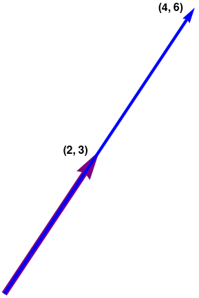
ar1 = Graphics[{Arrowheads[0.15], Thickness[0.03], Purple,
Arrow[{{0, 0}, {2, 3}}]}];
ar2 = Graphics[{Arrowheads[0.08], Thickness[0.015], Blue,
Arrow[{{0, 0}, {4, 6}}]}];
txt1 = Graphics[
Text[Style["(2, 3)", FontSize -> 16, Black, Bold], {1.5, 3}]];
txt2 = Graphics[
Text[Style["(4, 6)", FontSize -> 16, Black, Bold], {3.5, 6}]];
Show[ar1, ar2, txt1, txt2, Axes -> True,
GridLines -> {{2, 4}, {3, 6}}]
|
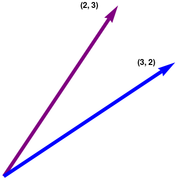
b. The vectors v and u are certainly not multiples of one another. Could they be linearly dependent? Suppose that there are scalars c₁ and c₂ satisfying \[ c_1 {\bf v} + c_2 {\bf u} = {\bf 0} . \] If c₁ ≠ 0, then we can solve for v in terms of u; that is, v = (−c₂/c₁)u, This is impossible because v is not a multiple of u. So c₁ must be zero. Similarly, c₂ must also be zero. Thus, {v, u} is linear independent set.
|
ar1 = Graphics[{Arrowheads[0.1], Thickness[0.02], Purple,
Arrow[{{0, 0}, {2, 3}}]}];
ar2 = Graphics[{Arrowheads[0.1], Thickness[0.02], Blue, Arrow[{{0, 0}, {3, 2}}]}]; txt1 = Graphics[ Text[Style["(2, 3)", FontSize -> 16, Black, Bold], {1.5, 3}]]; txt2 = Graphics[ Text[Style["(3, 2)", FontSize -> 16, Black, Bold], {2.5, 2}]]; Show[ar1, ar2, txt1, txt2] |
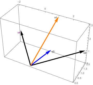
v1 = {1, 2, 3};
v2 = {3, 2, 1};
v3 = {1, 1, 1};
v4 = {-2, 2, 1};

|
But the plot of all four looks like they are all independent.
vecs1 = Graphics3D[{Thickness[0.01], Arrowheads[Large],
Arrow[{{0, 0, 0}, v2}], Arrow[{{0, 0, 0}, v4}],
Arrow[{{0, 0, 0}, v1}], Arrow[{{0, 0, 0}, v3}]}, Axes -> True]
|
|
This improves when we add color to the two suspect vectors
vecs2 = Graphics3D[{{Arrowheads[0.06], Thickness[0.01],
Arrow[{{0, 0, 0}, v2}], Purple}, {Arrowheads[0.06],
Thickness[0.01], Arrow[{{0, 0, 0}, v4}], Red}, {Arrowheads[0.06],
Thickness[0.01], Orange,
Arrow[{{0, 0, 0}, v1}]}, {Arrowheads[0.06], Thickness[0.01], Blue,
Arrow[{{0, 0, 0}, v3}]}, Text["v1", {.9*1, .9*2, 3}],
Text["v3", {1.2*1, .9*1, 1}], Purple, Text["v4", {-2, .9*2, .9*1}],
Black, Text["v2", {3, 2, .8*1}]}, Axes -> True]
|
|
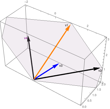
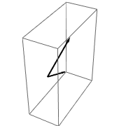
It improves further by adding a plane showing v1 and v3 together
infPl = Graphics3D[{Opacity[.2],
InfinitePlane[{{0, 0, 0}, v1, v3}, Mesh -> True]}];
vecs3 = Show[vecs2, infPl, ViewPoint -> {1.5346926334477773`, -2.116735802004978, 2.148056811481361}] |

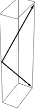
|
It helps to rotate the box so that the plane disappears, visually, to become a line. However, when we do that it appears that not two but THREE of our vectors are in the same plane (note the black arrowhead of v2 appears to be colinear with v1 and v3)
vecs4 = Show[vecs2, infPl,
ViewPoint -> {2.5066082420449374`,
0.103322560978032, -2.2707354688085837`}]
|
Let p be the largest power of x in such a linear combination—we want to know if there exists (not all zero) scalars c₀, c₁, c₂, … , cp such that \[ c_0 + c_1 x + c_2 x^2 + \cdots + c_p x^p = 0 . \tag{9.1} \] By plugging x = 0 into that equation, we see that c₀ = 0. Setting p = 10 in Mathematica, we get
% /. x -> 0
c₀ = 0
Taking the derivative of both sides of Equation (9.1) then reveals that \[ c_1 + 2\,c_2 x + 3\, c_3 x^2 + \cdots + p\,c_p x^{p-1} = 0 , \] and plugging x = 0 into this equation gives c₁ = 0. By repeating this procedure (i.e., taking the derivative and then plugging in x = 0), we similarly see that c₁ = c₂ = ⋯ = cp = 0, so S is linearly independent.
Again, for example, using p = 10
% /. x -> 0
c₁ = 0
Homogeneous Equations as Vector Combinations
To find a linear dependence relation among v₁, v₂, and v₃, completely row reduce the augmented matrix and write the new system \[ \begin{bmatrix} 2 & 5 & 1 & 0 \\ 6 & 8 & 3 & 0 \\ 2 & 4 & 1 & 0 \end{bmatrix} \,\sim\, \begin{bmatrix} 2 &\phantom{-}0 & 1 & 0 \\ 0 & -7& 0 & 0 \\ 0 & \phantom{-}0 & 0 & 0 \end{bmatrix} . \] This yields \[ \begin{split} 2\,x_1 \phantom{2x3} + x_3 &= 0 , \\ \phantom{-12} - 7\, x_2 \phantom{2x3}&= 0 , \\ 0&= 0 . \end{split} \] Thus, 2x₁ + x₃ = 0 and x₂ = 0. This yields the linear dependence equation: \[ {\bf v}_1 + 0\,{\bf v}_2 - 2\,{\bf v}_3 = {\bf 0} . \] We verify our conclusion with Mathematica:
v1 = {2, 6, 2};
v2 = {5, 8, 4};
v3 = {1, 3, 1};
b = {0, 0, 0};
MatrixForm[%]
MatrixForm[%]
-
Are the sets of two vectors {v, u}, {v, w}, {v, z}, {u, w}, {u, z}, and {w, z} each linearly independent?
Solution: We know from Corollary 3 that two vectors are linearly dependent if and only if one of them is a constant (scalar) multiple of another. Since every pair consists of not parallel vectors, every subset of two vectors is linearly independent.
Below we see a graphical portrayal of the six pairs of vectors, clearly none are parallel
Clear[v, u, w, z];Then we define the vectors:
sset2 = Subsets[{v, u, w, z}, {2}]v = {1, 2, 3}; u = {1, 3, -4}; w = {1, 2, -3}; z = {-2, 7, -5};
set = {v, u, w, z};{{{1, 2, 3}, {1, 3, -4}}, {{1, 2, 3}, {1, 2, -3}}, {{1, 2, 3}, {-2, 7, -5}}, {{1, 3, -4}, {1, 2, -3}}, {{1, 3, -4}, {-2, 7, -5}}, {{1, 2, -3}, {-2, 7, -5}}}ssets = Drop[Subsets[set, 2], 5]{{{1, 2, 3}, {1, 3, -4}}, {{1, 2, 3}, {1, 2, -3}}, {{1, 2, 3}, {-2, 7, -5}}, {{1, 3, -4}, {1, 2, -3}}, {{1, 3, -4}, {-2, 7, -5}}, {{1, 2, -3}, {-2, 7, -5}}}Grid[{ssets[[;; 3]], Map[Graphics3D[{Thick, Arrow[{{0, 0, 0}, ssets[[#, 1]]}], Arrow[{{0, 0, 0}, ssets[[#, 2]]}]}] &, Range[3]], ssets[[4 ;; 6]], Map[Graphics3D[{Thick, Arrow[{{0, 0, 0}, ssets[[#, 1]]}], Arrow[{{0, 0, 0}, ssets[[#, 2]]}]}] &, {4, 5, 6}]}, Frame -> All](1, 2, 3), (1, 3, −4) (1, 2, 3), (1, 2, −3) (1, 2, 3), (−2, 7, −5) 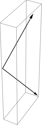
Although usually we do need termwise matrix division or multiplication, sometimes it is convenient to perform term by term arithmetic operations on matrices. This example provides a proper choice for term by term division of matrices (of course, of the same dimensions) and Mathematica supports these arithmetic operations. For example, we can divide or multiply term-by-term matrices, For instance, we define 2 × 3 matrices and divide or multiply them term-by-term:(1, 3, −4), (1, 2, −3) (1, 3, −4), (−2, 7, −5) (1, 2, −3), (−2, 7, −5) 

 A = {{1, 2}, {3, 4}, {5, 6}}; B = {{2, 3}, {1, 4}, {-1, -2}};
A/B{{1/2, 2/3}, {3, 1}, {-5, -3}}or multiplyA*B{{2, 6}, {3, 16}, {-5, -12}}Since vectors constitute a particular case of matrices, we can divide vectors of the same size element by element. If any pair of vectors is linearly dependent, then their division produces a vector of the same scalar multiple. This is not the case below so we conclude there are no scalar dependencies between these pairs.v = {1, 2, 3}; u = {1, 3, -4}; w = {1, 2, -3}; z = {-2, 7, -5};
set = {v, u, w, z};
ssets = Drop[Subsets[set, 2], 5]
(#[[1]]/#[[2]]) & /@ ssets{{1, 2/3, -(3/4)}, {1, 1, -1}, {-(1/2), 2/7, -(3/5)}, {1, 3/2, 4/ 3}, {-(1/2), 3/7, 4/5}, {-(1/2), 2/7, 3/5}} -
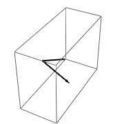
Is the set of four vectors {v, u, w, z} linearly dependent?
Solution: From Corollary 4, it follows that these four vectors of size 3 are linearly dependent.
Grid[{set, Map[Graphics3D[{Thick, Arrow[{{0, 0, 0}, set[[#]]}], Arrow[{{0, 0, 0}, set[[#]]}]}] &, Range[4]]}, Frame -> All]Adding a plane to our plot is not determinative unless we change the viewpoint such that the plane disappears.
Plane of vectors. infPl = Graphics3D[{Opacity[.4], InfinitePlane[{{0, 0, 0}, u, w}, Mesh -> True]}]; vecsUW = Graphics3D[{Thick, Arrow[{{0, 0, 0}, u}], Arrow[{{0, 0, 0}, w}]}]; Show[infPl, vecsUW, ViewPoint -> {1.7677868473826688`, -1.813323932632412, 2.244278498217939}]Show[infPl, vecsUW, ViewPoint -> {0.8398423137197476, -2.7043140351649644`, 1.8523904791635182`}] -
We consider the following sets of three vectors: S₁ = {v, u, w}, S₂ = {v, u, z}, S₃ = {v, w, z}, S₄ = {u, w, z}. Determine which of these four sets is linearly dependent.
Solution: In order to determine whether set S₁ is linearly dependent or independent, we consider the system of homogeneous equations with respect to unknown constants c₁, c₂, and c₃: \[ c_1 {\bf v} + c_2 {\bf u} + c_3 {\bf w} = {\bf 0} . \] We rewrite it in coordinate form: \[ c_1 \left[ \begin{array}{c} 1 \\ 2 \\ 3 \end{array} \right] + c_2 \left[ \begin{array}{c} \phantom{-}1 \\ \phantom{-}3 \\ -4 \end{array} \right] + c_3 \left[ \begin{array}{c} \phantom{-}1 \\ \phantom{-}2 \\ -3 \end{array} \right] = \left[ \begin{array}{c} 0 \\ 0 \\ 0 \end{array} \right] \] Equating their three coordinates, we obtain the system of linear equations: \[ \begin{split} c_1 \phantom{2}+ c_2 \phantom{3}+ \phantom{2}c_3 &= 0 \qquad \Longrightarrow \qquad c_1 + c_3 = - c_2 , \\ 2\, c_1 + 3\,c_2 + 2\,c_3 &= 0 \qquad \Longrightarrow \qquad c_2 = 0 , \\ 3\, c_1 -4\, c_2 - 3\, c_3 &= 0 \qquad \Longrightarrow \qquad c_1 - c_3 = 0. \end{split} \] Since this system has only trivial solution c₁ = c₂ = c₃ = 0, set S₁ is linearly independent.
Mathematica can solve this system in a number of ways, all of which produce the same answer.
LinearSolve[{Subscript[c, 1], Subscript[c, 2], Subscript[c, 3]} Subscript[s, 1], {0, 0, 0}]{0, 0, 0}Solve[{Subscript[c, 1], Subscript[c, 2], Subscript[c, 3]}.Subscript[s, 1] == 0, {Subscript[c, 1], Subscript[c, 2], Subscript[c, 3]}]{{Subscript[c, 1] -> 0, Subscript[c, 2] -> 0, Subscript[c, 3] -> 0}}Reduce[{Subscript[c, 1], Subscript[c, 2], Subscript[c, 3]}.Subscript[ s, 1] == 0, {Subscript[c, 1], Subscript[c, 2], Subscript[c, 3]}]Subscript[c, 1] == 0 && Subscript[c, 2] == 0 && Subscript[c, 3] == 0AugmentedMatrix[{}, vars_] := {} AugmentedMatrix[matA_List == matB_List, vars_] := AugmentedMatrix[matA - matB, vars] AugmentedMatrix[mat_, vars_] := With[{temp = CoefficientArrays[Flatten[Thread /@ mat], vars]}, Normal[Transpose[Join[Transpose[temp[[2]]], -{temp[[1]]}]]]]AugmentedMatrix[ \( \displaystyle \begin{pmatrix} 1&1&1 \\ 2&3&2 \\ 3&-4&-3 \end{pmatrix} \cdot \begin{pmatrix} c_1 \\ c_2 \\ c_3 \end{pmatrix} == \begin{pmatrix} 0 \\ 0 \\ 0 \end{pmatrix} , \) {c₁, c₂, c₃}];
MatrixForm[%]\( \displaystyle \begin{pmatrix} 1&1&1&0 \\ 2&3&2&0 \\ 3&-4&-3&0 \end{pmatrix} \)RowReduce[augM1];
MatrixForm[%]\( \displaystyle \begin{pmatrix} 1&0&0&0 \\ 0&1&0&0 \\ 0&0&1&0 \end{pmatrix} \)For S₂, we have to solve the system of homogeneous equations: \[ c_1 {\bf v} + c_2 {\bf u} + c_3 {\bf z} = {\bf 0} , \] which we rewrite as \[ c_1 \left[ \begin{array}{c} 1 \\ 2 \\ 3 \end{array} \right] + c_2 \left[ \begin{array}{c} \phantom{-}1 \\ \phantom{-}3 \\ -4 \end{array} \right] + c_3 \left[ \begin{array}{c} -2 \\ \phantom{-}7 \\ -5 \end{array} \right] = \left[ \begin{array}{c} 0 \\ 0 \\ 0 \end{array} \right] \] This leads to the system of linear equations: \[ \begin{split} c_1 \phantom{2}+ c_2 \phantom{3} -2\,c_3 &= 0 \qquad \Longrightarrow \qquad c_1 + c_2 = 2\, c_3 , \\ 2\, c_1 + 3\,c_2 + 7\,c_3 &= 0 \qquad \Longrightarrow \qquad 11\,c_1 + 13\,c_2 = 0 , \\ 3\, c_1 -4\, c_2 - 5\, c_3 &= 0 \qquad \Longrightarrow \qquad c_1 - 13\,c_2 = 0. \end{split} \] Since this system has only trivial solution, we claim that the set S₂ is linearly independent.
LinearSolve[{Subscript[c, 1], Subscript[c, 2], Subscript[c, 3]} Subscript[s, 2], {0, 0, 0}]{0, 0, 0}Let us consider the set S₃. In order to determine whether this set is linearly dependent or independent, we consider the system of homogeneous equations with respect to unknown constants c₁, c₂, and c₃: \[ c_1 {\bf v} + c_2 {\bf w} + c_3 {\bf z} = {\bf 0} , \] which we rewrite as \[ c_1 \left[ \begin{array}{c} 1 \\ 2 \\ 3 \end{array} \right] + c_2 \left[ \begin{array}{c} \phantom{-}1 \\ \phantom{-}2 \\ -3 \end{array} \right] + c_3 \left[ \begin{array}{c} -2 \\ \phantom{-}7 \\ -5 \end{array} \right] = \left[ \begin{array}{c} 0 \\ 0 \\ 0 \end{array} \right] \] The corresponding system of algebraic equations is \[ \begin{split} c_1 \phantom{2}+ c_2 \phantom{3} -2\,c_3 &= 0 \qquad \Longrightarrow \qquad c_1 + c_2 = 2\, c_3 , \\ 2\, c_1 + 2\,c_2 + 7\,c_3 &= 0 \qquad \Longrightarrow \qquad 11\,c_1 + 13\,c_2 = 0 , \\ 3\, c_1 -3\, c_2 - 5\, c_3 &= 0 \qquad \Longrightarrow \qquad c_1 - 13\,c_2 = 0. \end{split} \] This system has only trivial solution, so set S₃ is linearly independent.
Solve[{Subscript[c, 1], Subscript[c, 2], Subscript[c, 3]}.Subscript[s, 3] == 0, {Subscript[c, 1], Subscript[c, 2], Subscript[c, 3]}]{{Subscript[c, 1] -> 0, Subscript[c, 2] -> 0, Subscript[c, 3] -> 0}}Finally, we consider the set S₄. We build the system: \[ c_1 {\bf u} + c_2 {\bf w} + c_3 {\bf z} = {\bf 0} , \] which we rewrite as \[ c_1 \left[ \begin{array}{c} \phantom{-}1 \\ \phantom{-}3 \\ -4 \end{array} \right] + c_2 \left[ \begin{array}{c} \phantom{-}1 \\ \phantom{-}2 \\ -3 \end{array} \right] + c_3 \left[ \begin{array}{c} -2 \\ \phantom{-}7 \\ -5 \end{array} \right] = \left[ \begin{array}{c} 0 \\ 0 \\ 0 \end{array} \right] \] The corresponding system of algebraic equations is \[ \begin{split} c_1 \phantom{2}+ c_2 \phantom{3} -2\,c_3 &= 0 \qquad \Longrightarrow \qquad c_1 + c_2 = 2\, c_3 , \\ 3\, c_1 + 2\,c_2 + 7\,c_3 &= 0 \qquad \Longrightarrow \qquad 13\,c_1 + 11\,c_2 = 0 , \\ -4\, c_1 -3\, c_2 - 5\, c_3 &= 0 \qquad \Longrightarrow \qquad 13\, c_1 + 11\,c_2 = 0. \end{split} \] The last two equations are the same, so we have \[ c_2 = - \frac{13}{11}\, c_1 , \qquad c_3 = - \frac{1}{11}\, c_1 . \] Therefore, the system S₄ is linearly dependent.
Reduce[{Subscript[c, 1], Subscript[c, 2], Subscript[c, 3]}.Subscript[ s, 4] == 0, {Subscript[c, 1], Subscript[c, 2], Subscript[c, 3]}]Subscript[c, 2] == -((13 Subscript[c, 1])/11) && Subscript[c, 3] == -(Subscript[c, 1]/11)augM4 = AugmentedMatrix[ \( \displaystyle \begin{pmatrix} 1&1&-2 \\ 3&2&7 \\ -4&-3&-5 \end{pmatrix} \cdot \begin{pmatrix} c_1 \\ c_2 \\ c_3 \end{pmatrix} == \begin{pmatrix} 0 \\ 0 \\ 0 \end{pmatrix} , \) {c₁, c₂, c₃}];
MatrixForm[%]\( \displaystyle \begin{pmatrix} 1&1&-2&0 \\ 3&2&7&0 \\ -4&-3&-5&0 \end{pmatrix} \)owReduce[augM4];
MatrixForm[%]\( \displaystyle \begin{pmatrix} 1&0&11&0 \\ 0&1&-13&0 \\ 0&0&0&0 \end{pmatrix} , \)
in order to determine whether these functions are linearly independent or dependent, we set a system of equations \[ c_1 \cos x + c_2 \cos x + c_3 \cos^2 x = 0 , \]
{c1, c2, c3}.{Cos[x], Cos[x], (Cos[x])^2}
On the other hand the set B = {cos(2x), sin²(x), cos²(x)} is linearly dependent. Since this set is finite, we want to determine whether or not there exist scalars c₁, c₂, c₃ ∈ ℝ (not all equal to 0) such that \[ c_1 \cos (2x) + c_2 \sin^2 x + c_3 \cos^2 x = 0. \] We implement the same approach and plug in x = 0, π/2, and 3π/2. This yields the system of equations: \[ \begin{cases} c_1 + c_3 &= 0 , \\ -c_1 + c_2 &= 0 , \\ -c_1 + c_2 &= 0 . \end{cases} \] This system has multiple solutions \[ c_2 = c_1 , \qquad c_3 = -c_1 , \] where c₁ is a free variable. In particular, we get a relation \[ \cos (2x) = \cos^2 x - \sin^2 x . \] This relation shows that these three functions are linearly dependent.
Spans of Vectors
If S is an infinite set, linear combinations used to form the span of S are assumed to be only finite.
-
Two vectors in ℝ² or ℝ³ are linearly independent if and only if (iff) they do not lie on the same line when they have the initial points at the origin. Otherwise, one would be a scalar multiple of the other.
vect2D[vec_] := Grid[{{"Linearly\nDependent", "Linearly\nDependent", "Linearly\nIndependent"}, {Graphics[{Thickness[.04], Red, Arrowheads[.15], Arrow[{{0, 0}, vec}], Thick, Blue, Arrow[{{0, 0}, 2 vec}], Text[Style["v1", Bold, Red], {.85, 1}*vec], Text[Style["v2", Bold, Blue], {1.8, 2} vec]}, Axes -> True], Graphics[{Thickness[.02], Red, Arrowheads[.15], Arrow[{{0, 0}, vec}], Thick, Blue, Arrow[{{0, 0}, -2 vec}], Text[Style["v1", Bold, Red], {.85, 1}*vec], Text[Style["v3", Bold, Blue], vec*{-1.7, -1}]}, Axes -> True], Graphics[{Thickness[.02], Red, Arrowheads[.15], Arrow[{{0, 0}, vec}], Thick, Blue, Arrow[{{0, 0}, {2, 2/3}*vec}], Text[Style["v1", Bold, Red], {.9, 1}*vec], Text[Style["v4", Bold, Blue], {1.8, 2/3}*vec]}, Axes -> True]}}, Frame -> All]; vect2D[{2, 3}]

Linearly dependent. 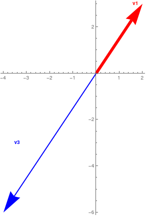
Linearly dependent. 
Independent. -
Three vectors in ℝ³ are linearly independent if and only if they do not lie in the same plane when they have their initial points at the origin. Otherwise, one would be a scalar multiple of the other.
Clear[v, gr1, gr2, gr3, plane1];
v = {2, 2, 2}; plane1 = Plot3D[3*a - 2*b, {a, -3, 4}, {b, -3, 4}, PlotStyle -> {Blue, Opacity[0.5]}, Axes -> True, Mesh -> None, Axes -> False]; gr1 = Graphics3D[{Black, Arrowheads[0.02], Thickness[0.01], Arrow[{{0, 0, 0}, v}], Arrow[{{0, 0, 0}, v*{-1, 1, -5}}], Arrow[{{0, 0, 0}, v*{.5, 1, .5}}], White, Text["v", v*{.85, 1.1, 1}], Text["u", v*{-.95, .8, -5}], Text["w", v*{.25, 1.05, .5}]}];gr2 = Graphics3D[{Black, Arrowheads[0.02], Thickness[0.01], Arrow[{{0, 0, 0}, v}], Arrow[{{0, 0, 0}, v*{-1, 1, -5}}], Arrow[{{0, 0, 0}, 2*v}], White, Text["v", v*{.85, 1.1, 1}], Text["u", v*{-.95, .8, -5}], Text["w1", {3.4, 2.9, 3.5}]}]; v1 = {2, 3, 5}; u1 = {-2, 4, -10}; gr3 = Graphics3D[{Black, Arrowheads[0.02], Thickness[0.01], Arrow[{{0, 0, 0}, v1}], Arrow[{{0, 0, 0}, u1}], Arrow[{{0, 0, 0}, w1}], White, Text["v1", {1.4, 2.9, 4.5}], Text["u1", {-2, 3.3, -10}], Text["w1", {3.7, 2.5, 3.5}]}];Grid[{{"Linearly\nDependent", "Linearly\nDependent", "Linearly\nIndependent"}, {Show[plane1, gr1], Show[plane1, gr2, PlotRange -> All], Show[plane1, gr3, PlotRange -> All, ViewPoint -> {-1.565, -1.627, 2.521}]}}, Frame -> All]GraphicsGrid[{{sh1, sh2, sh3}}, Frame -> All, ImageSize -> 1200]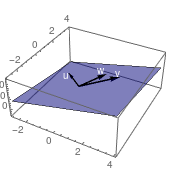
Plane with linearly dependent. 
Plane with two vectors. 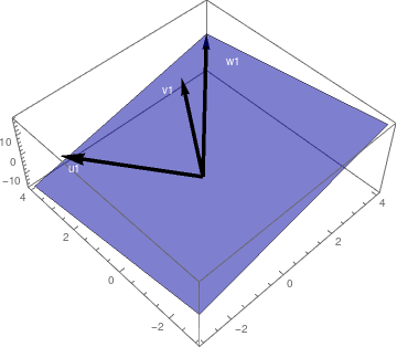
Independent vectors.
Theorem 2: Every spanning set S of a vector space V must contain at least as many elements as any linearly independent set of vectors from V.
Theorem 3: The span of any subset S of a vector space V is a subspace of V. Moreover, any subspace of V that contains S must also contain the span of S.
If S ≠ ∅, then S contains an element z. So 0z = 0 is an element of span( S ). Let x,y ∈ span( S ). Then there exist elements u1, u2, ... , um, v1, v1, ... , vn, in S and scalars a1, a2, ... , am, b1, b2, ... , bn such that
Now let W denote any subspace of V that contains S. If w ∈ span( S ), then w has the form w = c1w1 + c2w2 + ... + ckwk for some elements w1, w2, ... , wk in S and some scalars c1, c2, ... , ck. Since S⊆W, we have w1, w2, ... , wk ∈ W. Therefore, w = c1w1 + c2w2 + ... + ckwk is an element of W. Since w, an arbitrary element of span( S ), belongs to W, it follows that span( S ) ⊆ W, completing the proof. ■
Theorem 4: Let S, T be nonempty subsets of a vector space V over a field 𝔽, then
- If S ⊆ T, then span(S) ⊆ span(T);
- span(span(S)) = span(S).
- Assume that S ⊆ T. Then S ⊆ T ⊆ span(T), and hence S ⊆ span(T). According to Theorem 3, the span of S is the smallest subspace of V containing S. So span(S) ⊆ span(T).
- Obviously span(S) ⊆ span(span(S)). Now let v ∈ span(span(S)). Then \( \displaystyle {\bf v} = \sum_{1 \le j \le m} c_j {\bf v}_j , \) with c ∈ 𝔽 and vj ∈ span(S)). On other hand, each of vj ∈ span(S) can be written as \( \displaystyle {\bf v}_j = \sum_{1 \le k \le p} b_{jk} {\bf u}_k , \) with bk ∈ 𝔽 and uk ∈ S. This shows that every vector v ∈ span(span(S)) can be expanded as a linear combination of elements uk ∈ S. Therefore, span(span(S)) ⊆ span(S).
Theorem 5: Let S be a linearly independent subset of a vector space V, and let v be an element of V that is not in S. Then \( S \cup \{ {\bf v} \} \) is linearly dependent if and only if v belongs to the span of the set S.
Conversely, let \( {\bf v} \in \mbox{span}(S) . \) Then there exist vectors v1, ... , vm in S and scalars b1, b2, ... , bm such that \( {\bf v} = b_1 {\bf v}_1 + b_2 {\bf v}_2 + \cdots + b_m {\bf v}_m . \) Hence,
The next example demonstrates how Mathematica can determine the basis or set of linearly independent vectors from the given set. Note that basis is not unique and even changing the order of vectors, a software can provide you another set of linearly independent vectors.
Then each of the following scripts determine a subset of linearly independent vectors:
Last @ QRDecomposition @ Transpose @ m ] ]]
or, using subroutine
Module[{tm, ntm, ytm, mm = x}, {tm = RowReduce[mm] // Transpose,
ntm = MapIndexed[{#1, #2, Total[#1]} &, tm, {1}],
ytm = Cases[ntm, {___, ___, d_ /; d == 1}]};
Cases[ytm, {b_, {a_}, c_} :> mm[[All, a]]] // Transpose]
MinimalSublist[m1]
You see 1 row and n columns together in m1, so you can transpose it to see it as column vector
- Are the following 2×2 matrices \( \begin{bmatrix} -3&2 \\ \phantom{-}1& 2 \end{bmatrix} , \ \begin{bmatrix} \phantom{-}6&-4 \\ -2&-4 \end{bmatrix} \) linearly dependent or independent?
-
In each part, determine whether the vectors are linearly independent or a
linearly dependent in ℝ³.
- (2 ,-3, 1), (-1, 4, 5), (3, 2, -1);
- (1, -2, 0), (-2, 3, 2), (4, 3, 2);
- (7, 6, 5), (4, 3, 2), (1, 1, 1), (1, 2, 3);
-
In each part, determine whether the vectors are linearly independent or
linearly dependent in ℝ4.
- (8, −9, 6, 5), (1,−3, 7, 1), (1, 2, 0, −3);
- (2, 0, 2, 8), (2, 1, 0, 6), (1, −2, 5, 8);
-
In each part, determine whether the vectors are linearly independent or a
linearly dependent in the space ℝ≤3[x] of all polynomials of degree up to 3.
- {3, x + 4, x³ −5x, 6}.
- {0, 2x, 3 −x, x³}.
- {x³ −2x, {x³ + 2x, x + 1, x −3}.
-
In each part, determine whether the 2×2 matrices are linearly
independent or linearly dependent.
- \( \begin{bmatrix} 1&\phantom{-}0 \\ 2& -1 \end{bmatrix} , \ \begin{bmatrix} 0&\phantom{-}5 \\ 1&-5 \end{bmatrix} , \ \begin{bmatrix} -2&-1 \\ \phantom{-}1&\phantom{-}3 \end{bmatrix} ; \)
- \( \begin{bmatrix} -1&0 \\ \phantom{-}1& 2 \end{bmatrix} , \ \begin{bmatrix} 1&2 \\ 2&1 \end{bmatrix} , \ \begin{bmatrix} 0&1 \\ 2&1 \end{bmatrix} ; \)
- ????????? \( \begin{bmatrix} -2&9 \\ \phantom{-}3& 5 \end{bmatrix} , \ \begin{bmatrix} \phantom{-}1&7 \\ -2&3 \end{bmatrix} , \ \begin{bmatrix} -2&8 \\ \phantom{-}4&9 \end{bmatrix} \)
-
Determine all values of k for which the following matrices are linearly
dependent in ℝ2,2, the space of all 2×2 matrices.
- \( \begin{bmatrix} 1&2 \\ 0& 0 \end{bmatrix} , \ \begin{bmatrix} k&0 \\ 4&0 \end{bmatrix} , \ \begin{bmatrix} -1&k-2 \\ \phantom{-}k&0 \end{bmatrix} ; \) ?????
- \( \begin{bmatrix} -1&9 \\ \phantom{-}3& 4 \end{bmatrix} , \ \begin{bmatrix} \phantom{-}5&6 \\ -3&1 \end{bmatrix} , \ \begin{bmatrix} -2&8 \\ \phantom{-}1&7 \end{bmatrix} \)
- \( \begin{bmatrix} -2&9 \\ \phantom{-}3& 5 \end{bmatrix} , \ \begin{bmatrix} \phantom{-}1&7 \\ -2&3 \end{bmatrix} , \ \begin{bmatrix} -2&8 \\ \phantom{-}4&9 \end{bmatrix} \)
-
In each part, determine whether the three vectors lie in a plane in
ℝ³.
- Coffee
- Tea
- Milk
-
Determine whether the given vectors v₁ , v₂ , and
v₃ form a linearly dependent or independent set in ℝ³.
- v₁ = (−3, 0, 4), v₂ = (5, −1, 2), and v₃ = (3, 3, 9);
- v₁ = (−4, 0, 2), v₂ = (3, 2, 5), and v₃ = (6, $minus;1, 1);
- v₁ = (0. 0. 1), v₂ = (0, 5, −8), and v₃ = (−4, 3, 1);
- v₁ = (−2, 3, 1), v₂ = (1, −2, 4), and v₃ = (2, 4, 1);
- v₁ = (−5, 7, 8), v₂ = (−1, 1, 3), and v₃ = (1, 4, −7).
- Determine for which values of k the vectors x² + 2x + k, 5x² + 2kx + k², kx² + x + 3 generate ℝ≤2[x]
- Given the vectors \[ {\bf v} = \begin{pmatrix} 2 \\ 2 \end{pmatrix}, \quad {\bf u} = \begin{pmatrix} 0 \\ 1 \end{pmatrix}, \quad {\bf w} = \begin{pmatrix} 1 \\ -1 \end{pmatrix}, \] determine if they are linearly independent and determine the subspace generated by them.
- Determine if x³ −x belongs to the span of the vectors span(x³ + x² + x, x² + 2x, x²).
-
Find the value of k for which the set of vectors is linearly dependent.
????????????????
- \( \begin{bmatrix} -2&4 \\ \phantom{-}4& 5 \end{bmatrix} , \ \begin{bmatrix} \phantom{-}6&7 \\ -1&8 \end{bmatrix} , \ \begin{bmatrix} -2&8 \\ \phantom{-}5&1 \end{bmatrix} \)
- \( \begin{bmatrix} -1&9 \\ \phantom{-}3& 4 \end{bmatrix} , \ \begin{bmatrix} \phantom{-}5&6 \\ -3&1 \end{bmatrix} , \ \begin{bmatrix} -2&8 \\ \phantom{-}1&7 \end{bmatrix} \)
- \( \begin{bmatrix} -2&9 \\ \phantom{-}3& 5 \end{bmatrix} , \ \begin{bmatrix} \phantom{-}1&7 \\ -2&3 \end{bmatrix} , \ \begin{bmatrix} -2&8 \\ \phantom{-}4&9 \end{bmatrix} \)
-
Are the vectors v₁ , v₂ , and
v₃ in part (a) of the accompanying figure linearly independent? What about those in part (b) ?
??????????????????????// Anton page 211, # 15
- Find the solution of the system with parameter k: \[ \begin{split} kx - ky + 2z &= 0, \\ x - z &= 1, \\ 2x + 3ky -11z &= -1. \end{split} \]
- Anton, Howard (2005), Elementary Linear Algebra (Applications Version) (9th ed.), Wiley International
- Beezer, R.A., A First Course in Linear Algebra, 2017.