The following definition gives important notation and terminology for constructing vector spaces. It is also widely used in other areas of mathematics, such as real analysis and differential equations.
George Hill
The term linear combination is due to the American astronomer and
mathematician George William Hill (1838--1914), who introduced it in a research paper on planetary motion published in 1900. Working out of his home in West Nyack, NY, independently and largely in isolation from the wider scientific community, he made major contributions to celestial mechanics and to the theory of ordinary differential equations. He taught at Columbia University for a few years. The importance of his work was explicitly acknowledged by Henri Poincaré in 1905.
In other words, a linear combination of vectors from S is a sum of scalar multiples of those vectors.
Observe that in any vector space V, 0v = 0 for each vector
v∈V. Thus, the zero vector is a linear combination of any nonempty subset of V. So a linear combination is an expression that defines another vector. In this
case, we say that a vector v is represented as a linear combination of
vectors from (finite) set S:
Example 1:
Our first example has a little connection to vector spaces, but it illustrates usefulness of the term of linear combination in real life.
It is well-known that the U.S. political system is binary---there are only two parties in charge of leading the country. This situation is a result of a plurality voting system that is used to determine a winner in any election. The majority of countries in the world except for a few (U.S., U.K., and in the lower house in India) do not use the plurality method for nationwide elections as it is easy to manipulate and it is self-contradicting (a loser can win election). Let us denote by r the vector (or basket) indicating the Republican party, and by b the corresponding vector for Democratic party. Then an election can be represented by v, their linear combination
\[
{\bf v} = x {\bf b} + y {\bf r} ,
\]
where x is the number of voters that prefer Democratic party candidate, and y is the number of voters for Republican party candidate. Note that in this example, scalars are taken from the set of nonnegative integers, denoted by ℕ, which is not a field.
■
Example 2:
Consider the following table that shows the vitamin content of 100 grams of 6
foods with respect to vitamins B1 (thiamine),
B2 (riboflavin), B3 (Niacin Equivalents),
C (ascorbic acid), and B9 (Folate).
B1 (mg)
B2 (mg)
B3 (mg)
C (mg)
Folate (mcg)
Watermelon
0.05 mg
0.03 mg
0.45 mg
12.31 mg
4.56 mcg
Honey
0.03 mg
0.038 mg
0.02 mg
1.7 mg
6.8 mcg
Pork
0.396 mg
0.242 mg
4.647 mg
0.3 mg
212 mcg
Salmon
0.02 mg
0.2 mg
6 mg
0
25 mcg
Lettuce
0.07 mg
0.08 mg
0.375 mg
9.2 mg
73 mcg
Tomato
0.528 mg
0.489 mg
5.4 mg
39 mg
20 mcg
The vitamin content of 100 grams of each food can be recorded as a column
vector in ℝ5; for example the vitamin vector for tomato is
Portions are a vector (where 𝑎₁ = Watermelon (W), 𝑎₂ = Honey (H), etc.
■
Example 3:
Humans distinguish colors due to special sensors, called cones, in their eyes.
Approximately 65% of all cones are sensitive to red light, 33% are sensitive
to green light, and only 2% are sensitive to blue (but the blue cones are the
most sensitive). Most color models in use today are oriented either toward
hardware (such as for color monitors and printers) or toward applications
where color manipulation is a goal (such as in the creation of color graphics
for animation).
Colors on computer monitors or video cameras are commonly based on what is called the RGB color model in which red, green, and blue light are added together in various ways to reproduce a broad array of colors.
Red is the color at the end of the visible spectrum of light, next to orange and opposite violet. It has a dominant wavelength of approximately 625–740 nanometers. Green is the color between blue and yellow on the visible spectrum. It is evoked by light which has a dominant wavelength of roughly 495–570 nm.
The human eye perceives blue when observing light with a dominant wavelength between approximately 450 and 495 nanometres.
The CMY (cyan, magenta, yellow) and CMYK (cyan, magenta, yellow, black) models are used for color printing.
Images represented in the RGB color model consist of three component images, one for each primary color. When fed into an RGB monitor, these three images combine on the screen to produce a composite color image. the number of bits used to represent each pixel in RGB space is called the pixel depth. Consider an RGB image in which each of the red, green, and blue images is an 8-bit image. Under these conditions each RGB color pixel, which is a triplet (R, G, B), is said to have a depth of 24 (= 3×8) bits. The total number of colors in a 24-bit RGB image is \( \left( 2^8 \right)^3 = 16,777,216. \) One way to identify the primary colors is to assign the vectors:
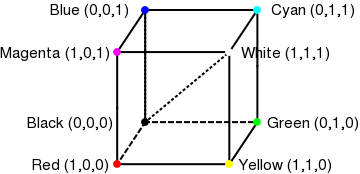
r = (1,0,0) pure red,
g = (0,1,0) pure green,
b = (0,0,1) pure blue
in ℝ³ and to create all other colors by forming linear combinations
of r, g, and b using coefficients between 0 and 1,
inclusive; these coefficients represent the percentage (gray scale) of each
pure color in the mix. The set of all such color vectors is called RGB color space or the RGB color cube. Thus, each color vector c in this cube is expressed as a linear combination of the form
where 0≤ak≤1. As indicated in the figure below, the cones
of the cube represent the pure primary colors together with the colors black,
white, magenta, cyan, and yellow. The vectors along the diagonal running from
black to white correspond to gray scale.
Example 4:
In a rectangular xy-coordinate system every vector in the plane can be
expressed in exactly one way as a linear combination of the standard unit
vectors. For example, the only way to express the vector (4,3) as a linear
combination of i = (1,0) and j = (0,1) is
As we see from the previous example, a vector may have several representations
in the form of linear combinations from the given set of vectors.
Example 5:
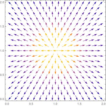
In 3-dimensional space, the electric field E of a point charge q1 with position vector r1 at a point P---called the field point---with position vector r is given by the formula
where ke is the universal Coulomb constant, ke = 8.99×10⁹N⋅m²/C², q is the charge of the particle.
We define the position vectors in Mathematica:
r = {x,y,z}; r1 ={x1,y1,z1} ;
When we place a semicolon at the end of an expression, Mathematica does not provide any
output. Next, we will write an expression for the field
(with ke = 1). Recall that in Mathematica
vector names are followed by underscores when being called in a
function.
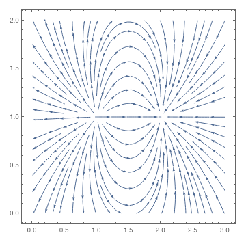
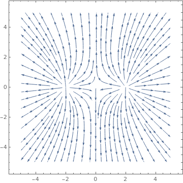
Let us see what the field lines of a dipole look like. A dipole is a combination of two charges of equal strength and opposite signs. Let the positive charge of +1 be at (1,1,0) and the negative charge of -1 be at (2,1,0). Let us also assume that the field point is at (x,y,0). Since we are interested in a two-dimensional plot of the field lines, we separate the first two components of Etotal
Example 6:
The vector [-2, 8, 5, 0] is a linear combination of the vectors [3, 1,
-2, 2], [1, 0, 3, -1], and [4, -2, 1 0], because it is the sum of
scalar multiples of the three vectors:
Both a vector and a matrix can be multiplied by a scalar; with the operation being *. Matrices and vectors can be added or subtracted only when their dimensions are the same.
Generators
Vector spaces can be generated from arbitrary sets.
Let A be a set, and 𝔽 a field. The free vector space over 𝔽 generated by
A is the vector space Free(A) consisting of all formal finite linear combinations of elements of A.
Example 7:
Let A = { ♠, ♦, ♣, ♥ } and 𝔽 = ℝ. Then the Free(A) over the field of real numbers is the four-dimensional
vector space consisting of all elements (𝑎♠, b♦, c♣, d♥), where 𝑎, b, c, d ∈ ℝ. Addition
and scalar multiplication are defined in the obvious way.
for k ∈ ℝ. Then four suits generate ordering of real components in ℝ4.
End of Example 7
■
Situation becomes more fruitful when we consider subset of a vector space instead of arbitrary set. Staring from a finite number of vectors v1, v2, … , vn from a vector space V, we can construct a vector subspace of V as follows. Consider the subset consisting of all (finite) linear combinations of these vectors. Actually, this subset of all linear combinations becomes a vector space---the smallest possible vector space containing the given subset of vectors.
The span of a set S of vectors, also called linear span, is the linear space formed by all the vectors that can be written as linear combinations of the vectors belonging to the given set. We also say that the set Sgenerates the vector space and denote it by span(S). Then W = span(S) is generated by S
and its elements are called generators of W.
Observation: A set of vectors generates (or span) a vector space if their linear combinations fill the space.
Although the definition of span has no restriction on the size of the generating set S, we will mostly work with finitely generated vector spaces. Moreover, we try to use as fewer generating vectors as possible. Any generating set of vectors can be enlarged indefinitely, say by adding kw (k is any scalar and wS) without changing the resulting span.
A vector space V is finitely generated when it has a finite generating family S of vectors: V = span(S) = span(v1, v2, … , vn).
Example 8:
The span of a single non-zero vector {v} consists of all constant multiples of this vector. This set is referred to as a line generated by v. If v = 0, zero vector, then its span consists of a single vector---0. We call this vector space a trivial space.
End of Example 8
Let S be a finite set of vectors. Its span, denoted by span(S), does not depend on the order in which elements of S are listed, Hence we call S a set, not a list. Its span is defined as
If W = span(S) is a span of a nonempty set S, we can enlarge S and include any linear combination w of elements from S. Then W = span(S∪{w}). Also, if any vector from the set S is a linear combination of other vectors from S, this vector can be removed from the generating set S without changing span(S).
The span is a subspace since the trivial combination (all coefficients are 0) produces
the zero vector of span(S). A multiple of a linear combination is again a linear combination:
When vectors are defined by arrays of numbers as above, it is assumed that they both start at the origin with tips indicated in Eq.(9.1).
These two vectors generate a plane through the origin:
\[
a\,x +b\,y + c\,z = 0,
\tag{9.2}
\]
for some real numbers 𝑎, b, and c. In order to identify these coefficients, we substitute into equation (9.2) both vectors to obtain
\[
\begin{split}
2 \left( a +b + c \right) &= 0,
\\
- 2 \, a + 2\,b -10\,c &= 0.
\end{split}
\tag{9.3}
\]
To solve this system of algebraic equations, we employ Mathematica:
$Post := If[MatrixQ[#1],
MatrixForm[#1], #1] & (* outputs matrices in MatrixForm*)
Clear[a, b, c, v, u];
v = {2, 2, 2};
u = {-2, 2, -10};
{x->-3 z y->2z}
The substitution is accomplished below by filling "#n" slots with the new variables, 𝑎, b, and c, respectively, shown in the square brackets in each equation.
Now, we substitute the values we just found for a and b into a slightly rearranged second equation of (9.3) and get a numeric value of c.
In the code below, the symbols "/." are interpreted by Mathematica as "given that..."
sol2 = Solve[-2*a + 2*b == -10 /. sol1, c]
{z -> -1}
Using this constant value for c in sol1 gives
sol3 = sol1 /. c -> -1
{a -> 3 b -> -2}
So we obtain the required values of coefficients that we use to define the equation of the plane:
\[
3\,x -2\,y -z = 0.
\tag{9.4}
\]
Another option to solve system of equations (9.3) is to add these two equations.
eq83a = v.{a, b, c}
eq83b = u.{a, b, c}
2 a +2b + 2 c
-2 a + 2 b 010 c
sol4 = eq83a + eq83b
4 b - 8 c
Setting this result equal to zero and solving for b provides its value in terms of c:
\[
4\, b - 8\, c = 0 \qquad \Longrightarrow \qquad b = 2\, c .
\]
sol5 = Solve[sol4 == 0, b]
{b -> 2 c}
Using this relation, we obtain from either of equations (9.3) that
\[
2\,a + 2\cdot 2\,c + 2\,c = 0 \qquad \Longrightarrow \qquad a = -3\, c .
\]
sol6 = eq83a /. sol5
{2 a + 6 c}
sol7 = Solve[sol6 == 0, a]
{a -> -3 c}
which leads to equation (8.4).
eq84 = Plus @@ {#1 a, #2 b, #3 c} &[sol3[[1, 1, 2]], sol3[[1, 2, 2]],
sol2[[1, 1, 2]]]
3 a - 2 b - c
Note that Mathematica delivers its solutions as "expressions" each of which is composed of "parts" represented in the code as "levels" enclosed by double square brackets . Thus, for example, the coefficient for "a" (above as slot #1) is the second element (3) of the first element (a\[RightArrow]3) of the solution's first element ({a\[RightArrow]3,b\[RightArrow]-2}) which is the entirety of sol3, each shown below in the order described here.
sol3[[1, 1, 2]]
3
sol3[[1, 1]]
a -> 3
sol3[[1]]
{a -> 3 b -> -2}
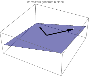
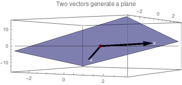
We are now in a position to illustrate our work graphically. This also provides a chance to check our work. The task is to represent a two dimensional abstraction, two vectors each on the same plane. But, because the plane itself is at an angle, we need to show our 2d abstraction using a three dimensional (3d) space.
We wish to believe two things: One is that both vectors lie upon the same plane; the other is that both vectors begin at the origin. They both start at the origin by construction, but whether picture conforms it, we want to verify. Viewing the graphic from above does not confirm this information. We can rotate the 3d box such that you view it from the side as if your head was at about the top of the southeast corner of the box. The plane nearly disappears. At that viewpoint the plane appears as a line which coincides with the two vectors. It looks very likely that the vectors lie upon the plane. This is known as a "conjecture." We need more evidence.
For our second hope, that the two vectors each begin at the origin, we will add two elements to our graphic. One is the "zero plane" for which all z values are zero, the other is a red point at the origin.
Two vectors generate a plane
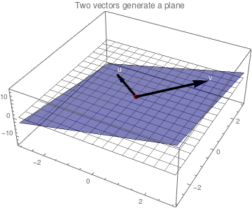
From above we can approximate the position of the origin and imagine that the red dot is that point with respect to the x and y axes. But the location of the red point relative to the z-axis is harder to see. Again, tilting the graphic such that the zero plane disappears into a line, below we see that the conjecture about our vectors may actually be true.
Two vectors generate a plane
Until now, we have used words like "conjecture," "wish to believe," "hope," "imagine," "increases our confidence," "may actually be true," and "need more evidence." These words, to mathematicians, constitute what is uncharitably referred to as "hand waving." The etymology of this term is interesting and leads to a lot of jokes involving mathematicians and engineers. All of the words suggest uncertainty and that is intentional.
Mathematicians prefer a formal proof relying on inductive reasoning, which follows a specific format (Definition, Theorem, Proof, Remarks) handed down over the centuries. Keywords in a proof are "let," "show," and a conclusion acronym "QED" which stands for "Quod Erat Demonstrandum," literally "Which was to be demonstrated" or colloquially "We proved it true and are through talking about it."
Such a proof is provided below:
We need to show that any vector from the plane (8.4) can be expressed as alinear combination of vectors (8.1):
The first equivalent relation is obtained upon subtraction of the first row from each of the two other rows. The last relation follows upon adding the second row times two with to the last row.
Therefore, this system (8.5) has a unique solution for any x, y ∈ ℝ:
\[
c_1 = \frac{1}{2} \left( y + x \right) , \qquad c_2 = \frac{1}{4} \left( y - x \right) .
\]
It is frustrating for students when a computer (or a Professor) skips steps and just produces the answer. Using Trace you can see each step of the Mathematica code execution
To examine the code (and the process) more closely, you can extract a line of code and evaluate it separately. Here I take the 6th line from the cell above and use the name assignments instead of the matrix and vector values to get the solution for an interim step.
trGauss[[1, 6]]
Last /@ RowReduce[Flatten /@ Transpose[{mat, vec}]]
Mathematica has a number of approaches to solving this problem, each resulting in the same answer:
The system (1) is consistent (or compatible) precisely when vector equation (2) is valid for suitable values of the coefficients xi, namely when b is a linear combination
of the vectors aj:
namely when the m-tuples a1, a2, … , an form a set of generators of 𝔽m.
Assume now that system (1) has infinitely many solutions (for a suitably given right-hand side b), but all have the same value xj for some fixed j. To fix ideas,
let us assume that x1 has the same value in all solutions of (1). By the basic principle of linear algebra, all solutions are obtained from a particular one, by
addition of a solution of
Hence x1 has a fixed value in all solutions of (2) when all solutions of (3)
have a zero value for x1. This simply means that a1 is not a linear combination
of a2, a3, … , an. Indeed, any expression
Hence it corresponds to a solution of (3) having a first coefficient
x1 = 1 ≠ 0.
In other
words, x1 has a fixed value in all solutions of (2) precisely when a1 is not a
linear combination of a2, a3, … , an, namely,
More generally, xj has a fixed value in all solutions of (1) precisely when aj is
not a linear combination of the other m-tuples.
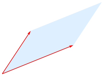
To illustrate how vectors define a space through their linear combinations,
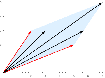
we pick up two non-collinear vectors u and v and plot them.
The figure below includes a parallelogram (in light blue) that illustrates our intention to include all linear combinations of two vectors u and v with positive coefficients of values less than one. So this parallelogram represents only a part of span of two vectors u and v.
u = {2, 3};
v = {5, 2};
vecArr = Graphics[{Thick, Red, Arrow[{{0, 0}, u}],
Arrow[{{0, 0}, v}]}];
poly = Graphics[{LightBlue, Polygon[{{0, 0}, u, u + v, v}]}];
Show[poly, vecArr]
Two vectors form a parallelogram.
Mathematica code
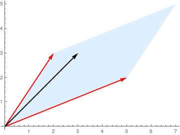
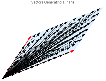
We now wish to see how vectors that are linear combinations of those u and v outlining vectors generate a space. Choosing coefficients a₁ = 1.5 and a₂ = 1, we multiply these, respectively, times the elements of u, creating a new vector
{1.5, 1}*u
{3., 3}
This creates the corresponding vector that can be visualized as an arrow; so we see that it fits within the span of u and v.
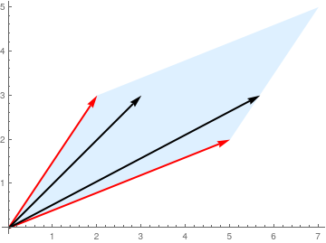
In order to demonstrate this linear combination phenomenon, we plot with Mathematica several combinations:
u = {2, 3};
v = {5, 2};
vecArr = Graphics[{Thick, Red, Arrow[{{0, 0}, u}],
Arrow[{{0, 0}, v}]}];
poly = Graphics[{LightBlue, Polygon[{{0, 0}, u, u + v, v}]},
PlotLabel -> "Vectors Generating a Plane"];
poly2 = DiscretizeRegion[Polygon[{{0, 0}, u, u + v, v}]];
polyMesh = Drop[MeshCoordinates@poly2, 4]; Animate[
If[end < 115,
Graphics[Table[Arrow[{{0, 0}, polyMesh[[i]]}], {i, 1, end}],
PlotLabel -> "Vectors Generating a Plane"],
Show[poly, vecArr,
Graphics[Table[Arrow[{{0, 0}, polyMesh[[i]]}], {i, 1, end}],
PlotLabel -> "Vectors Generating a Plane"]]],
{{end, 1, "Add Vectors"}, 1, 115},
AnimationRepetitions -> 1
]
A part of span of two non-collinear vectors.
Remark:
It is important to keep in mind that linear combinations are
always finite, even if itds generating set is not. To illustrate this point, consider the vector space ℝ[x] = span(1, x, x², x³, …), which is the set of all polynomials (of any degree). Recall from calculus that we can represent the function sin(x) in the form
We have written sin(x) as a sum of scalar
multiples of 1, x, x², x³, and so on. However sin(x) is not a polynomial in x because sin(x) can only be written as an infinite sum of polynomials, not a finite one.
Which of the following are linear combinations of two vectors v = (1, 2, −1) and u = (3, 0, 1)?
\[
({\bf a}) \quad (1, 1, 1), \qquad ({\bf b}) \quad (-3, 6, -5) , \qquad ({\bf c}) \quad (3 , 2, 1).
\]
Which of the following are linear combinations of three vectors v = (1, 2, −1), u = (1, 1, 1), and w = (3, 0, 1)?
\[
({\bf a}) \quad (3, -5, 3), \qquad ({\bf b}) \quad (-6, 5, -4) , \qquad ({\bf c}) \quad (3 , 2, 1).
\]
Express the following as linear combinations of b>v = (−1, 2, 4), u = (1, −3, 1), and w = (3, 1, 2).
\[
({\bf a}) \quad (-10, 7, -1), \qquad ({\bf b}) \quad (8, 1, -11) , \qquad ({\bf c}) \quad (3 , 22, 7).
\]