Duality is a complex notion having ramifications in many topics of mathematics and physics.
The notion of a dual space is useful because we can phrase many important concepts in linear algebra without the need to introduce
additional structure. In particular, we will see that we can formulate many notions involving
inner products in a way that does not require the use of an inner product because ⟨φ|v⟩ can be thought of as the action of a linear functional ⟨φ| on ket vector |v⟩.
In addition, it allows us to view subspaces
as solutions of sets of linear equations and vice-versa.
When we speak about duality, it is understood as a duality with respect to what? This section gives an introduction to this important topic and mostly consider basic duality concepts with respect to the field of scalars 𝔽.
To some extent, a duality can be viewed as a property to see an object similar to the original picture when it is applied twice, analogous to a mirror image. For instance, in real life, when a person is married, his wife can be considered as a dual image with respect to "marriage operation;" however, her marriage leads to second duality---a husband, who can be the same if it is the first marriage, or it can be another husband due to the second marriage. Another example of duality provides de Morgan's laws.
A special type of duality provides involution operations; when J : V ⇾ V and J² = J ⚬ J = I, the identity operation. So marriage is not always an involution, but complex conjugate is.
When an inner product is employed, it forms a special structure in vector space that should be taken into account by duality. We discuss duality of Euclidean spaces in Part V.
Dual Spaces
Recall that the set of all linear transformations from one vectors space V into another vector space W is denoted as ℒ(V, W). Its particular case arises when we choose W = 𝔽 (as a one-dimensional coordinate vector space over itself).
Let V be an 𝔽-vector space over a field 𝔽 (which is either ℝ or ℂ or ℚ). A linear functional
(also known as linear form or covector)
on V is a linear map V ⇾ 𝔽. In other words, a linear
functional T on V is a scalar-valued function that satisfies
for any vectors u, v ∈ V and any scalars α, β ∈ 𝔽.
Linear functionals can be thought of as giving us snapshots of vectors—knowing
the value of φ(v) tells us what v looks like from one particular direction or
angle (just like having a photograph tells us what an object looks like from
one side), but not necessarily what it looks like as a whole.
Alternatively, linear forms can be thought of as the building blocks that
make up more general linear transformations. Indeed, every linear
transformation into an n-dimensional vector space can be thought of
as being made up of n linear forms (one for each of the n output dimensions).
Our first example, which seem a trivial one, clarifies the concept of duality. Let V = ℂ be the set of all complex numbers over the field ℂ (itself). We consider the involution operation
So J maps the complex plane into itself by swapping it with respect to the abscissa (called the real axis in ℂ). Note that we denote complex conjugate by z* instead of overline notation \( \displaystyle \overline{z} = \overline{x + {\bf j}\,y} = x - {\bf j}\,y , \) which is common in mathematics literature. As you see, the asterisk notation is in agreement with notation of dual spaces. When V is considered as a complex vector space, then complex conjugate convolution is not a linear operation because
However, when V = ℂ is considered as a vector space over the field of real numbers, J is a linear transformation.
Example 1:
Let us consider fruit inventory in a
supermarket, assuming that there are αa apples, αb bananas, αc coconuts, and so on. We designate it as a vector
Fruit inventories like these form a space V that resembles a vector space, It is closed under addition and scalar multiplication (by rational numbers). V is not truly a vector space because we don't define subtraction or multiplication by negative numbers. Basis elements \( \hat{e}_i \) maybe considered as different containers because fruits are not allowed to be mixed.
Next, we consider a particular purchase price function, $p. Its values yield the cost of any fruit inventory x:
Thus, this purchase price function is a linear functional:
\[
\$_p \, : \, V \mapsto \mathbb{R} ,
\]
which provides a measurement (in dollars) of any fruit inventory (vector x∈V).
Example 2:
We consider several familiar vector spaces and linear functions on these spaces.
Let V be ℝ², a Cartesian product of two real lines. We consider a functional T : V ↦ ℝ, defined by
\[
T({\bf u}) = T(x,y) = x + 2\,y .
\]
We leave it to the reader to prove that T is a linear function.
Let ℭ[𝑎, b] be a set of all continuous functions on closed interval [𝑎, b]. For any function f ∈
ℭ[𝑎, b], we define a functional T on it by
\[
T(f) = \int_a^b f(x)\,{\text d} x .
\]
When you studied calculus, you learned that T is a linear function.
You can define another linear functional on
ℭ[𝑎, b]:
\[
T(f) = f(s) , \qquad s \in [a, b],
\]
where s is an arbitrary (but fixed) point from the interval.
This functional can be generalized to obtain a sampling function. Let { s1, s2, … , sn } ⊂ [𝑎, b] be a specified collection of points in [𝑎, b], and let { k1, k2, … , kn } be a set of scalars. Then the function
\[
T(f) = \sum_{i=1}^n k_i f(s_i )
\]
is a linear function on V.
Let us consider the set of all square matrices over some field 𝔽, which we denote by V = 𝔽n,n. Then evaluating a trace of any square matrix is a linear functional on V.
Let us consider a set ℘[t] of all polynomials in variable t of finite degree, which is a vector space over a field of constants 𝔽. Let k1, k2, … , kn be any n scalars and let t1, t2, … , tn be any n real numbers. Then the formula
\[
T(p) = \sum_{i=1}^n k_i p(t_i )
\]
defines a linear functional on ℘[t].
End of Example 2
We observe that for any linear functional φ acting on any vector space V,
That is why a linear functional is sometimes called homogeneous.
In particular, for any vector v = (v1, v2,… , vn) ∈ ℂn
and any set of n complex numbers k1, k2,… , kn ∈ ℂ, the formula
Theorem 1:
Let V be an n-dimensional space with a basis β = { e1, e2, … , en }. If { k1, k2, … , kn } is any list of n scalars, then there is one and only one linear functional φ on V such that φ(ei) = < φ | ei > = ki for i = 1, 2, … , n.
Every v in V may be written in the form v = s1e1 + s2e2 + ⋯ + snen in one and only one way because β is a basis. If ψ is any linear functional, then
then ψ is indeed a linear functional and <ψ|ei> = ki.
Example 3:
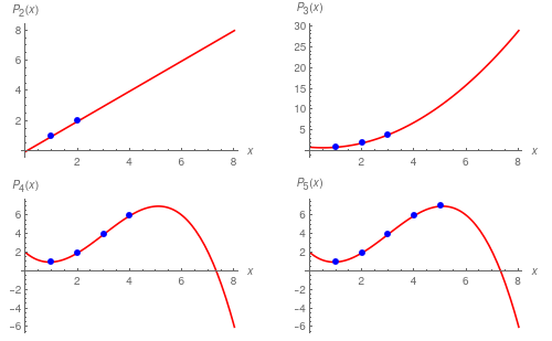
Let 𝑎1, 𝑎2, … , 𝑎n+1 be distinct points (in
ℝ or ℂ), and let ℝ≤n[x] be the space of polynomials of degree at most n in variable x. Define
n+1 linearly independent functionals
where j in the products runs from 1 to n + 1. Since the numerator of polynomial pk(x is a product of simple monomials (x − 𝑎j) that vanish at x = 𝑎j, we have pk(𝑎k) = 1 and
pk(𝑎j) = 0 if j ≠ k, so indeed the system p1(x), p2(x) , … , pn+1(x) is dual to the system φ1, φ2, … , φn+1.
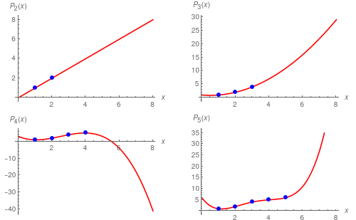
Now we can construct a polynomial that makes specified values at the given list of points 𝑎1, 𝑎2, … , 𝑎n+1:
Note in the output below, each graphic has a different label for each y axis as the k in Subscript[p, k] increments higher; and the number of points coincide with the value of the k subscript. Accordingly, the product of these approaches the true functional form with added increments.
A set of all linear functions ℒ(V, 𝔽) deserves a special label.
The dual space of V, denoted by V*, is the vector space of all linear functionals on V, i.e., V* = ℒ(V, 𝔽).
When dealing with linear functionals, it is convenient to follow Paul Dirac (1902--1984) and use his bra-ket notation (established in 1939). In quantum mechanics, a vector v is written in abstract ket form as |v>. A linear functional φ is written in bra form as <φ|, it is also frequently called a covector. Then a functional φ acting on vector v is written as
rather than traditional form φ(v) utilized in mathematics. So a bra-vector acts according to some linear law on a ket-vector to give a scalar output.
For any ground field 𝔽, the bra-ket notation establishes the bilinear mapping
Dirac's notation \eqref{EqDual.1} provides a duality between a vector space V and its dual space V*. A most important example of a linear functional provides the dot product when 𝔽 = ℝ:
This is actually the “standard” example of a linear form, and
the one that we should keep in mind as our intuition builders. We will see shortly
that every linear functional on a finite-dimensional vector space can be written in this way.
Since bra-ket notation resembles an inner product, it is common to consider
kets as column vectors, and bras are identified with row vectors. Then you can multiply 1×n matrix <φ| (which is a row vector) with n×1 matrix |v> (which is column vector) to obtain a 1×1 matrix, which is isomorphic to a scalar. Strictly speaking, this operation should be written as <φ|·|v> or, dropping the dot for multiplication, <φ| |v>, but double vertical lines are substituted with a single one. Moreover, Dirac's notation allows us to combine bras, kets, and linear operators (they are matrices in finite dimensional case) together and interpret them using matrix multiplication:
\[
< \varphi\, |\, {\bf A}\,|\, {\bf v} > ,
\]
where A is an operator acting either on ket vector v (from left to right) or on covector (= bra) <φ| (from right to left).
This naturally leads to inner product (see section in Part 5). Bra–ket notation is also known as Dirac notation, despite the notation having a precursor in Hermann Grassmann's use of [ ϕ ∣ ψ ] for inner products nearly 100 years earlier.
A definite state of a physical system is represented as a state ket or state vector. However, we can get physical information about the system only upon some measurement. This is achieved by applying a bra vector so we could get physically relevant information about the system by combining bras with kets.
In short, the state ket as such gives relevant information about the system only upon measurement of observables, which is accomplished by taking the product of bras and kets.
We consider here only finite-dimensional spaces because for infinite-dimensional spaces the
dual space consists not of all but only of the so-called bounded linear functionals. Without giving
the precise definition, let us only mention than in the finite-dimensional case (both the domain
and the target space are finite-dimensional) all linear transformations are bounded, and we do not
need to mention the word bounded (or continuous).
Theorem 2:
The set V* is a vector space.
The dual set is obviously closed under two operations: addition between functionals and multiplication by a scalar. Therefore, we need to check all eight axioms that are used for vector space definition.
φ + ψ = ψ + φ for φ, ψ ∈ V*;
φ + (ψ + χ) = (ψ + φ) +χ for φ, ψ, χ ∈ V*;
the zero element is the constant zero function;;
the additive inverse of ψ is −ψ ∈ V*;
(ks)ψ = k(sψ) for ψ ∈ V* and k, s ∈ 𝔽;
1ψ = ψ ∈ V*;
k(φ + ψ) = kφ + kψ for φ, ψ ∈ V* and k ∈ 𝔽;
(k + s)ψ = kψ + kψ for k, s ∈ 𝔽 and ψ ∈ V*.
Example 4:
Let the space V be ℝn, what is its dual? To answer this question we replace the direct product ℝn = ℝ × ℝ × ⋯ × ℝ by its isomorphic image ℝn×1 of column vectors. So instead of n-tuples we consider column vectors that are matrices of size n × 1. Then
a linear transformation T : ℝn,1 ⇾ ℝm,1 is represented by an m × n
matrix. Therefore, it is convenient to identify ℝn with n-dimensional column vector space ℝn,1, then a linear functional on ℝn ≌ ℝn,1 (i.e., a linear transformation φ : ℝn ⇾ ℝ)
is given by an 1 × n matrix (a row); we denote it by bra-vector. The collection
of all such rows is isomorphic to ℝn,1 (isomorphism is given by taking the transpose of a ket-vector).
So, the dual of ℝn is ℝn itself. The same holds true for ℚn or ℂn, of course, as
well as for 𝔽n, where 𝔽 is an arbitrary field. Since the space V over a field 𝔽 (we use only either ℚ or ℝ or ℂ) of dimension n is
isomorphic to 𝔽n, and the dual to 𝔽n is isomorphic to 𝔽n, we can conclude
that the dual V* is isomorphic to V.
Remember that identifying the direct product 𝔽n with column vector space 𝔽n,1 and its dual space with row vector space 𝔽1,n is just a convenient assumption that will remind you matrix multiplication. From mathematical and computational point of view a 1 × 1 matrix is not the same as a scalar, but it is isomorphic to this scalar. Mathematica distinguishes these two objects:
a = {{1, 2}}.{3, 1}
{5}
SameQ[a, 5]
False
For a bra vector ⟨φ∣ = [φ1, φ2, … , φn], the action
on a ket-vector ∣v⟩ = [v1, v2, … , vn] ∈ 𝔽n is given by dot product
Suppose that V is finite-dimensional and let β = { e1, e2, … , en }
be a basis of V. For each i = 1, 2, … , n, define a linear functional ej : V ↦ 𝔽 by setting
It is customary to denote dual bases in V* by the same letters as corresponding bases in V but using lower indices ("downstairs") for V and upper indices ("upstairs") for V*. Then vectors v = viei in V can be represented
by objects vi with an upper index, and dual vectors φ = φiei in V* by objects vi with a lower index. It is convenient to use the Einstein summation convention and drop the summation symbol ∑. In this language, the canonical isomorphism between V and V* is realized by
lowering and raising indices. Upper index objects vi represent coordinate vectors relative to a basis ei of V and are also called covariant vectors.
Lower index objects φi are the coordinates of dual vectors relative to the dual basis ei and are also called contravariant vectors.
Theorem 3:
The set β* is a basis of V*. Hence, V* is finite-dimensional and dimV* = dimV.
First we check that the functionals { e1, e2, … , en } are linearly independent. Suppose that there exist 𝔽-scalars k1, k2, … , kn so that
Note that the 0 on the right denotes the zero functional; i.e., the functional that sends
everything in V to 0 ∈ 𝔽. The equality above is an equality of maps, which should hold
for any v ∈ V we evaluate either side on. In particular, evaluating both sides on every element from the basis β, we have
Again, this means that both sides should give the same result when evaluating on any v ∈ V. By linearity, it suffices to check that this is true on the basis β. Indeed, for each i, we get
again by the definition of the ei and the bi. Thus, φ and b1e1 + ⋯ + bnen agree on the basis, so
we conclude that they are equal as elements of V*. Hence {e1, e2, … , en} spans V* and therefore
forms a basis of V*.
Example 5:
In vector space ℝ³, let us consider a (not orthogonal) basis
Since a vector space V and its dual V* have the same dimension, hence, they are isomorphic. In general, this isomorphism depends on a choice of bases. However, a canonical isomorphism (known as Riesz representation theorem) between V and its dual V* can be defined if V carries a
non-degenerate inner product.
Theorem 4:
If v and u are any two distinct vectors of the n-dimensional vector space V, then there exists a linear functional φ on V such that <φ|v> ≠ <φ|u>; or equivalently, to any nonzero vector v ∈ V, there corresponds a ψ ∈ V* such that
<ψ|v> ≠ 0.
This theorem contains two equivalent statements because we can always consider the difference u − v to reduce the first statement to the homogeneous case. So we prove only the latter.
Let β = { e1, e2, … , en } be any basis in vector space V, and let β* = { e1, e2, … , en } be the dual basis inV*. If
\( {\bf v} = \sum_i k_i {\bf e}_i , \) then <ej|v>; = ki. Hence, if <ψ|v> = 0 for all ψ, in particular, if <ej|v> = 0 for all j = 1, 2, … , n, then v = 0.
Example 6:
Let V = ℭ[0, 1] be the set of all continuous functions on the interval [0, 1]. Let f and g be two distinct continuous functions on the interval. Then there exists a point 𝑎 ∈ [0, 1] such that f(𝑎) ≠ g(𝑎). Let us consider a linear functional δ𝑎 that maps these two functions f and g into different real values. Indeed, let
\[
\delta_a (f) = f(a) ,
\]
Then δ𝑎 is a required functional that distinguishes f and g. As it is widely used in applications, the functional above can be written with the aid of Dirac delta function:
\[
\int_0^1 \delta (x-a)\,f(x)\,{\text d} x = f(a) .
\]
End of Example 6
From Theorem 4, it follows that a functional on any finite-dimensional vector space is unique; this means that if φ(v) = 0 for every v ∈ V, then φ ≡ 0.
Corollary 1:
Let φ ∈ V* be a nonzero functional on V, and let v ∈ V be any element such that φ(v) = <φ|v> ≠ 0.Then V is a direct sum of two subspaces:
Let v ∈ V be a vector that is not annihilated by linear form φ(v) = <φ|v> ≠ 0. Then we can choose a basis β of V such that β = { e1 = v, e2, … , en }, so that the first vector in this set is v. Let β* = { e1, e2, … , en } be a dual basis in V*. By definition of dual basis, e1(v) = 1, and for all other basis elements, we have
e1(ej) = 0, j = 2, 3, … , n. We can prove that kerφ⊂span{e2, … , en} and span{e2, … , en}⊂kerφ, so kerφ=span{e2, … , en}.
Therefore, the kernel (or null space) of e1 is n − 1 dimensional.
Hence, the functional φ has the following representation in the dual basis:
\[
\phi = \phi ({\bf v})\,{\bf e}^1 = c\, {\bf e}^1 , \qquad c\ne 0.
\]
This functional maps the rest basis elements { e2, … , en } to zero, so V = span(v) ⊕ kerφ because every vector v has a unique representation
\[
{\bf v} = {\bf v} = {\bf e}_1 + 0\cdot {\bf e}_2 + \cdots + 0\cdot{\bf e}_n .
\]
Example 7:
We identify the two dimensional vector space ℂ² of ordered pairs (z₁, z₂) of two complex numbers with its isomorphic image of column vectors:
We consider a linear form
\[
\varphi \left( z_1 , z_2 \right) = z_1 - 2{\bf j}\, z_2 .
\tag{7.1}
\]
As usual, j denotes a unit imaginary vector in ℂ, so j² = −1.
The kernel of φ consists of all pairs of complex numbers (z₁, z₂) for which z₁ = 2jz₂. Hence, the null space of φ is spanned on the vector
\[
\mbox{ker}\varphi = \left\{ \left[ \begin{array}{c} 2{\bf j}\,y \\ y \end{array} \right] : \quad y \in \mathbb{C} \right\} .
\tag{7.2}
\]
Let z = (z₁, z₂) be an arbitrary vector from ℂ²,and v = (1+j, 1−j) be given. We have to show that there is a unique decomposition:
\[
{\bf z} = \left( z_1 , z_2 \right) = c\left( 1 + {\bf j}, 1 - {\bf j} \right) + \left( 2{\bf j}, 1 \right) y ,
\tag{7.3}
\]
where y∈ℂ is some complex number. Equating two components, we obtain two complex equations:
\[
\begin{split}
z_1 &= c \left( 1 + {\bf j} \right) + 2{\bf j}\, y ,
\\
z_2 &= c \left( 1 - {\bf j} \right) + y .
\end{split}
\tag{7.4}
\]
Since the matrix of system (7.4) is not singular,
\[
{\bf A} = \begin{bmatrix} 1 + {\bf j} & 2{\bf j} \\ 1 - {\bf j} & 1 \end{bmatrix} \qquad \Longrightarrow \qquad \det{\bf A} = -1-{\bf j} \ne 0 ,
\]
1 + I - 2*I*(1 - I)
-1 - I
system (7.4) has a unique solution for any input z = (z₁, z₂):
\[
c = \frac{1 + {\bf j}}{2} \left( z_1 - 2{\bf j}\, z_2 \right) , \qquad y = - z_2 - {\bf j}\, z_1 .
\]
{{c -> (-(1/2) + I/2) (z1 - 2 I z2), y -> -I (z1 - I z2)}}
End of Example 7
■
In other words, any vector v not in the kernel of a linear functional generates a supplement of this kernel: The kernel of a nonzero linear functional has codimension 1. When V is finite dimensional, the rank-nullity theorem claims:
If a vector space V is not trivial, so V ≠ {0}, then its dual V* ≠ {0}.
Corollary 2:
Let φ, ψ be linear functionals on a vector space V. If φ vanishes on kerψ, then φ = cψ is a constant multiple of ψ.
If ψ = 0, there is nothing to prove. Let us assume that ψ ≠ 0, and
choose a vector x ∈ V such that ψ(x) ≠ 0. Consider the linear functional ψ(x)φ − φ(x)ψ,
which vanishes on x and on kerψ by assumption. By Corollary 1, this linear functional vanishes identically: We get a linear dependence relation.
Another proof:
∀ ϕ ∈ V∗, ∃ x such that ϕ(x) ≠ 0, according to Corollary 1, V = span(x) ⊕ kerϕ ⇒ ∀ v ∈ V, v = cx + y, y ∈ kerϕ ⇒ ψ(v) = ψ(cx + y) = ψ(cv) + ψ(y) = cψ(x) + 0 = c ψ(x)/ϕ(x ) ϕ(x) + ϕ(y) = ψ(x)/ϕ(cx ) ϕ(x) +ψ(x)/ϕ(x ) ϕ(y) = ψ(x)/ϕ(x ) ϕ(cx + y) = ψ(x)/ϕ(x ) ϕ(v).
Example 8:
We consider V = ℝ3,3, the set of all real-valued 3×3 matrices, and φ a linear functional on it:
where tr(M) is the trace of matrix M. The dimension of V is 9. Functional φ annihilates matrix M if and only if its trace is zero:
\[
a_{11} + a_{22} + a_{33} = 0 ,
\]
which imposes one condition (linear equation) on the coefficients of matrix M. Therefore, the kernel (null space) of φ is 8-dimensional (9 − 1 = 8). The image of φ is just ℝ, that is, one-dimensional vector space.
Trace is the sum of the diagonal elements in a matrix. Here is how Mathematica computes the Trace.
Theorem 5:
Let φi ∈ V* (1 ≤ i ≤ m)
be a finite set of linear functionals. If a linear functional ψ ∈ V* vanishes on intersection \( \displaystyle \cap_{1 \leqslant i \leqslant m} \mbox{ker}\varphi_i , \) then ψ
is a linear combination of the φi, so ψ ∈ span(φ1, … , φm).
Let us proceed by induction on m, noting that for m = 1, it is the
statement of Corollary 2. Let now m ≥ 2, and consider the subspace
\[
W = \cap_{i \leqslant i \leqslant m} \mbox{ker}\varphi_i \supset W \cap \mbox{ker}\varphi_1 ,
\]
as well as the restrictions of ψ and φ1 to W. By assumption, \( \displaystyle \left. \psi\right\vert_{W} \) vanishes on
kerφ1|W. Hence there is a scalar c such that
ψ|V = cφ1|V, namely,
ψ − cφ1 vanishes on W. By the induction assumption, ψ − cφ1 is a linear combination of φ2, … , φm, say
Example 9:
Let ℝ≤n[x] be a set of polynomials in variable x of degree up to n with real coefficients. As we know, the monomials ek(x) = xk (k = 0, 1, 2, … , n)) form a standard basis in this space.
where \( \displaystyle n^{\underline{j}} = n \left( n-1 \right) \left( n-2 \right) \cdots \left( n-j+1 \right) \) is the j-th falling factorial. As usual, we denote by \( \displaystyle \texttt{D}^0 = \texttt{I} \) the identity operator, and 0! = 1. It is not hard to check that ej form a dual basis for monomials xi. Indeed, substituting p(x) = xk into Eq.(8.1), we get
This polynomial expansion is well-known in Calculus as the Maclaurin formula.
(The Maclaurin formula is represented as a form of Taylor Series in Mathematica.)
■
The Dual of a Dual Space
In several areas of mathematics, isomorphism appears as a very general concept. The word derives from the Greek "iso", meaning “equal”, and "morphosis", meaning “to form” or “to shape.” Informally, an isomorphism is a map that preserves sets and relations among elements. When this map or this correspondence is established with no choices involved, it is called canonical isomorphism.
The construction of a dual may be iterated. In other words, we form a dual space \( \displaystyle \left( V^{\ast} \right)^{\ast} \) of the dual space V*; for simplicity of notation, we shall denote it by
V**.
We prefer to speak of a function f (not mentioning its variable), keeping f(x) for the image of x under this map. This approach is very convenient when dealing with linear functionals. For example, Dirac's delta function
\[
\delta_a \,:\ f \,\mapsto f(a)
\]
is a linear functional on a set of test functions.
The second dual V** is canonically (i.e., in a natural way) isomorphic to V. This means that any vector v ∈ V canonically defines a linear functional δv on V* (i.e. an element of the second dual V**) by the rule:
Note, that the null space of T is ker(T) = {0} due to uniqueness of linear functional. Finally, letting the element v vary in 𝔽-vector space V, we obtain a linear map
Theorem 6:
The linear map δ : V ⇾ V**, defined by v ↦ δv (φ ↦ φ(v), is injective function. When V is finite dimensional, it is a canonical isomorphism.
The meaning of δv = 0 is φ(v) = δv(φ) = 0 for all linear functionals φ. It implies that v = 0 due to Corollary 2. Hence, kerδ = {0}, so the linear map \eqref{EqDual.4} is injective. In the finite-dimensional case, we have
Example 10:
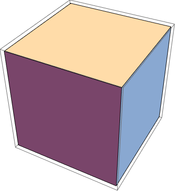
The "dual" of a vector is the linear transformation that it encodes onto the real or complex number. Another way of expressing the same concept is: the "dual" of a linear transformation from space to one dimension (ℂ or ℝ) is a certain vector in that space. A non-mathematician might, as a result of this, ascribe somewhat magical properties to the dot product because that is just what the dot product does: locate an answer to a vector question on the real number line or complex plane. Mathematicians and physicists have long studied the notion of Duality and have given various interpretations of it. One of these is that when two different mathematical abstractions share [some] properties, they are endowed with a correspondence that is very useful in practice. More complex transformations, such as Fourier, permit one to make theoretical progress on otherwise intractable problems in the transform space, achieving a result otherwise not possible and then transform that result back to the original for a practical answer that was out of reach in the pre-transformed expression.
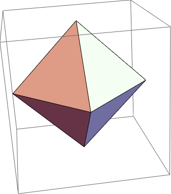
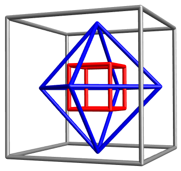
The figure below is a simple example of duality and how one may move easily from one to the other and back. Notice the commonality of six and eight in each figure. Each object has a set of 6 somethings and a set of eight somethings, but they are not the same things. For the cube it is six faces and eight vertices. Count the equivalent for the octahedron. Note the each have the same number of edges. There is a mathematical relation between the cube and the octahedron which permits one to "convert" one shape to the other; reversing that process returns to the original shape. Naturally, there is a scale factor involved, explaining why the outside cube is much larger than the one inside. The mathematical relationship is described above where the center of the faces of one are linked, thereby creating the other.
Since dimV** = dimV* = dimV, the condition ker(T) = {0} implies that
T is an invertible transformation (isomorphism).
The isomorphism T is very natural because it was
defined without using a basis, so it does not depend on
the choice of basis. So, informally we say that V** is canonically isomorphic
to V; the rigorous statement is that the map T described above (which we consider to be a natural and canonical) is an isomorphism from V to V**.
When we defined the dual space V* from V, we did so by picking a special basis (the dual basis), therefore, the isomorphism from V to V* is not canonical because it depends on the basis.
Since the dual space is intuitively the space of “rulers” (or measurement-instruments) of our vector space, and as so there is no canonical relationship between rulers and vectors because measurements need scaling, and there is no canonical way to provide one scaling for space.
On the other hand, the isomorphism \eqref{EqDual.4} between the initial vector space V and its double dual V** is canonical since mapping \eqref{EqDual.4} does not depend on local basis.
If we were to calibrate the measure-instruments, a canonical way to accomplish it is to calibrate them by acting on what they are supposed to measure.
Example 11:
A typical linear programming problem that was first formulated by the Russian scientist Leonid Kantorovich in 1939, asks to minimize the cost function c • x subject to constraints:
where A is an m × n matrix with real coefficients and b ∈ ℝm. As usual, the cost function c • b = c1x1 + ⋯ + cnxn is a dot product of two vectors. Any vector satisfying the constraint conditions is called feasible.
Theorem A:
If rhe feasible region is unbounded and the coefficients of the objective function are positive, then the minimum value of the objective function exists. Moreover, the minimum value of the objective function occurs at one (or more) of the corner points at the boundary of the feasible region.
The dual problem starts from the same A, b, and c, and reverses everything. In the primary problem, c is in the cost function and b is in the constraint, In the dual, b and c are
switched, The dual unknown y ∈ 𝔽1, m is a row vector with m components, and the feasible set
has yA ≤ c instead of Ax ≥ b.
In short, the dual of a minimum problem is a maximum problem. Now y ≥ 0:
\[
{\bf y}\,{\bf A} \le {\bf c}
\tag{11.2}
\]
The dual of this problem is the original minimum problem. There is complete symmetry
between the primal and dual problems. The simplex method applies equally well to a
maximization—anyway, both problems get solved at once.
Theorem B:
When both optimization problems have feasible vectors, they have
optimal solutions x* and y*, respectively. The minimum cost c • x* equals the maximum income y* • b.
If optimal vectors do not exist, there are two possibilities: Either both feasible sets are
empty, or one is empty and the other problem is unbounded (the maximum is +∞ or the
minimum is −∞).
End of Example 11
Annihilators
Recall that V is an 𝔽-vector space over field 𝔽 (which is either ℚ or ℝ or ℂ). The set of all linear functionals is denoted by V*.
If S is a subset (not need to be a subspace) of a vector space V, then the annihilatorS0 is the set of all linear functionals φ such that φ(v) = <φ|v> = 0 for all v ∈ S. When V is a Euclidean space, then its annihilator is denoted by S⊥.
From this definition, we immediately get that {0}0 = V* and V0 = {0}. If V is finite-dimensional and contains a non-zero vector, then Theorem 4 assures us that S0 ≠ V*.
Theorem 7:
If S is an m-dimensional subspace of an n-dimensional vector space V, then S0 is an (n−m)-dimensional subspace of V*.
then their sum is also an annihilator. Also, if we multiply φ by a constant c, then (cφ)(v) = c·φ(v) = c·0 = 0. So the set of all annihilators for arbitrary set S is a vector space.
Let β = { x1, x2, … , xn } be a basis in V whose first m elements are in S (so they constitute a basis in S as being linearly independent). Let β* = { y1, y2, … , yn } be the dual basis in
V*, We denote by R ⊂ V* the subspace spanned on { ym+1, ym+2, … , yn }. Clearly, R has dimension n−m. We are going to show that R = S0.
If x is any vector in S, then x is a linear combination of the first m elements from the basis β:
In other words, each yj, j = m+1, m+2, … , n, is in S0. It follows that R is in V*,
\[
R \subset S^0 .
\]
Now we prove the opposite relation and assume that y is any element of S0. Then it is a linear combination of vectors from the dual basis β*:
\[
{\bf y} = \sum_{j=1}^n b_j {\bf y}^j .
\]
Since by assumption, y is in S0, we have, for every i = 1, 2, … , m,
\[
0 = \langle {\bf y} \,|\,{\bf x}_i \rangle = \sum_{j=1}^n b_j \langle {\bf y}^j \,|\,{\bf x}_i \rangle = b_i .
\]
In other words, y is a linear combination of ym+1 , … , yn. This proves that y is in R and consequently that
\[
S^0 \subset R,
\]
and the theorem follows.
Theorem 8:
If S is a subspace of a finite-dimensional vector space V, then S00 = S.
By definition of S0, ⟨φ | x⟩ = 0 for all x ∈ S and all φ ∈ S0, it allows that S ⊂ S00, The desired conclusion follows from the dimension argument, Let S be m-dimensional, then dimension of S0 is n−m, and that of S00 is n − (n − m) = m. Hence S = S00.
Example 12:
Let V = ℝ≤n[x] be the space of polynomials of degree at most n in variable x. Let us consider its subset S that consists of all polynomials without a free term, so S = xℝ≤n-1[x]. Then its annihilator becomes
\[
S^0 = \left\{ \varphi \in V^{\ast} \, : \ \varphi (p) = p(0), \quad p \in V \right\} .
\]
Theorem 9:
Let X and Y be subspaces of a vector space V = X ⊕ Y. Then the dual space X* is isomorphic to
Y⁰ and Y* is isomorphic to
X⁰; moreover, V* = X⁰ ⊕ Y⁰.
The second annihilator consists of all polynomials p such that φ(p) = p(0) = 0. A polynomial to be zero at the origin should be without a free ter.
Let x ∈ X, φ ∈ X*, and x⁰ ∈ X⁰, respectively. Similarly, let y ∈ Y, ψ ∈ Y*, and y⁰ ∈ Y⁰. The subspaces X⁰ and Y⁰ are disjoint because if κ(x) = κ(y) = 0 for all x and y, then
κ(v) = κ(x + y) = 0 for all v
Moreover, if κ is any functional over V and if v = x + y, we write x⁰(v) = κ(y) and y⁰(v) = κ(x). It is not hard to see that functions x⁰ and y⁰ thus defined are linear functionals on V, so x⁰ and y⁰ belong V*; they also belong to X⁰ and Y⁰, respectively. Since κ = x⁰ + y⁰, it follows that V* is indeed the direct sum of X⁰ and Y⁰.
To establish the asserted isomorphisms, we make a correspondence to every x⁰ a functional ψ from Y* defined by ψ(y) = x⁰(y). It can be shown that the correspondence x⁰ ↦ ψ is linear and one-to-one, and therefore an isomorphism between X⁰ and Y*. The corresponding result for Y⁰ and X* follows from symmetry by interchanging x and y.
Example 13:
Hyperplanes
Example 14:
Let us consider the set V = ℂ of complex numbers as a real vector space. In this space, addition is defined as usual and multiplication of a complex number z = x + jy by a real number k is defined as kz = kx + jky. Here j is the unit imaginary vector on the complex plane, so j² = −1.
Consider the following functions and your task is to identify which of them is a linear functional on V = ℂ.
Let
v1, v2,… , vn+1
be a system of vectors in 𝔽-vector space V such that there exists a dual system v1, v2,… , vn+1 of linear functionals such that
\[
{\bf v}^j \left( {\bf v}_i \right) = \langle {\bf v}^j \, | \, {\bf v}_i \rangle = \delta_{i,j} .
\]
Show that the system v1, v2,… , vn+1 is linearly independent.
Show that if the system v1, v2,… , vn+1 is not generating, then the “biorthogonal” system" v1, v2,… , vn+1 is not unique.
Define a non-zero linear functional φ on ℚ³ such that if x₁ = (1, 2, 3) and x₂ = (−1, 1, −2), then ⟨φ | x₁⟩ = ⟨φ | x₂⟩ = 0.
The vectors x₁ = (3, 2, 1), x₂ = (−2, 1, −1), and x₃ = (−1, 3, 2) form a basis in ℝ³. If { e¹, e², e³ } is the dual basis, and if x = (1, 2, 3), find ⟨e¹ | x⟩ and ⟨e² | x⟩.
Prove that is φ is a linear functional on an n-dimensional vector space V, then the set of all those vectors for which ⟨φ | x⟩ = 0 is a subspace of V; what is the dimension of that subspace?
If φ(x) = x₁ + 2x₂ + 3x₃ whenever x = (x₁, x₂, x₃) ∈ ℝ³, then φ is a linear functional on ℝ³. Find a basis of the subspace consisting of all those vectors x for which ⟨φ | x⟩ = 0.
If R and S are subspaces of a vector space V, and if R ⊂ S, prove that S0 ⊂ R0.
Prove that if S is any subset of a finite-dimensional vector space, then S00 coincides with the subspace spanned on S.
If R and S are subspaces of a finite dimensional vector space V, then (R ∩ S)0 = R0 + S0 and (R + S)0 = R0 ∩ S0.
Prove the converse: given any basis β* = { φ1, φ2, … , φn } of V*, we can construct a dual basis { e1, e2, … , en } of V so that the functionals φ1, φ2, … , φn
serve as coordinate functions for this basis.
Consider ℝ³ with basis β = {v₁, v₂, v₃}, where v₁ = (−1, 4, 3), v₂ = (3, 2 −2), v₃ (3, 2 0). Find the dual basis β*.