This section provides a connection between ancient comprehension of vectors as quantities having magnitude and direction and vectors as arrays of numbers, presented in Part1 of this tutorial.
The classical (geometrical) model of vectors is assumed to provoke curiosity, incite mathematical intuition, and prepare the beginner for
the rigorous formalisms that follow.
Motivation
Quantities that completely specified by single data, like length, density, or
mass, are called scalars. In this tutorial, we consider only scalars that are elements of three fields: ℚ (rational numbers), ℝ (real numbers), or ℂ (complex numbers). Quantities that are not scalars, but that can be added and multiplied by scalas are referred to as vectors.
The concept of a vector in its earliest manifestation comes from physical considerations. In particular, there is evidence of velocity being thought as a vector---a quantity with direction and magnitude---in ancient Greek times. For instance, the treatise Mechanice by an unknown author in the fourth century B.C. is written: "When a body is moved in a certain ratio (i.e., has two linear movements in a constant fraction of one to another) the body must move in a
straight line, and this straight line is the diagonal of the parallelogram formed from the straight lines which have the given ratio." Heron of Alexandria (first century A.D.) gave a proof of this result when the directions were perpendicular. He showed that if a point P moves with a constant velocity over a line PQ while at the same time the line PQ moves with constant velocity along the parallel lines PR and QS so that it always remains parallel to its original position, and that if the time P takes to reach Q is the same as the time PQ takes to reach RS, then in fact the point P moves along the diagonal PS.
This basic idea of adding two motions vectorially was generalized from velocities to physical forces in the sixteenth and seventeenth centuries. One example of this practice is found the Law of Motion in Isaac Newton's Principia, where he shows that "a body acted on by two forces simultaneously will describe the diagonal of a parallelogram in the same time as it would describe the sides by those forces separately."
Before invention of rectangular coordinates in 1637 by the French philosopher, scientist, and mathematician René Descartes (1596--1650) (Latinized name: Cartesius),
geometrical prospective dominated (including name "vector"). Since 85% of information comes to humans through eyes, developing a geometric intuition cannot be ignored.
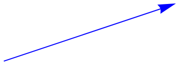
Physicists have found a very useful geometric interpretation of forces acting on a body. The motion in response to a force depends on the direction in which the force is applied and on the magnitude of the force---that is, on how hard the force is exerted. It is natural to represent a force by an arrow, pointing in the direction in which the force is acting, and with the length of the arrow representing the magnitude of the force. Such an arrow is a force vector. In short, a vector is a term that refers colloquially to some quantities that cannot be expressed by a single number, but can be fully characterized by its magnitude and direction.
It leads naturally to describe a vector as an arrow, which is a graphical symbol, such as ← or →, or a pictogram, used to point or indicate direction.
However, the arrow symbol first appered in an illustration of Bernard Forest de Bélidor's treatise printed in France in 1737. The arrow is here used to illustrate the direction of the flow of water and of the water wheel's rotation. Usage of arrows in mathematics originated in 1922 by David Hilbert (1862--1943).
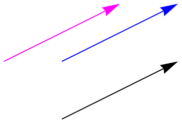
In most physical situations involving vectors,
only the magnitude and direction of the vector are significant; consequently,
we regard vectors with the same length and direction as being equal (or equivalent) irrespective to their positions.
When we think of vectors as arrows, they are not based at the origin
necessarily; a vector is simply the direction and the magnitude, and it does not know where it starts. A vector whose point of application is not fixed but magnitude and direction is, is called free vector. Fixed or localised vector is whose point of application is fixed.
Same vector can become free or fixed depending on scenario. Like if a force F is applied on a table which has rotational and translational motion. If we are Interested in Translational motion then we consider force F as free vector because we can move it to the centre of mass of the table in solving the problem.
While solving rotational motion of the table, the point of application of force F is fixed since torque has to be calculated.
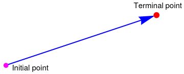
It is a custom to visualize vectors with arrows (geometric object on the plane or 3D space). The tail of
the arrow is called the initial point of the vector and the
tip the terminal point. To emphasis this approach, an arrow
is placed above the initial and terminal points, for example, the notation
\( {\bf v} = \vec{AB} \) tells us that A is
the starting point of the vector v and its terminal point is
B. In this tutorial (as in most science papers and textbooks), we will
denote vectors in boldface type applied to lower case letters such as
v, u, or x.
In applications, people deal with a variety of quantities that are used to describe the physical world. Examples of
such quantities include distance, displacement, speed, velocity, acceleration, force, mass, momentum, energy, work,
power, etc. All these quantities can by divided into two categories -- vectors and scalars.
--->
The Cartesian coordinate system provides a natural generalization of vectors to higher dimensions independently of their geometrical interpretation of having magnitude and direction.
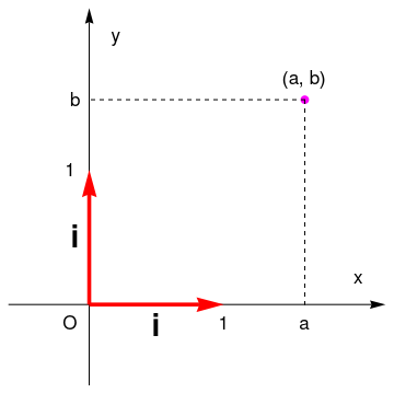
Using a rectangular coordinate system in the plane, note that if we consider a force vector to start from the origin (0, 0), then the vector is completely determined by the coordinates of the point at the tip of the arrow. Hence, we can consider each ordered pair in ℝ×ℝ to represent a vector in the plane as well as a point in the plane. When we wish to regard an ordered pair as a vector, we will use square brackets, rather than parentheses, to indicate this. Also, we often will write vectors as columns of numbers rather than as rows, and brackets notation is traditional for columns. Thus, we speak of the point (2, 1) in ℝ×ℝ and of the vector [2, 1] in ℝ₂ or vector \( \displaystyle \begin{bmatrix} 2 \\ 1 \end{bmatrix} \) in ℝ².
To represent the point (2, 1) in the plane, we make a dot at the appropriate place, whereas if we wish to represent the vector [2, 1], we draw an arrow emanating from the origin with its tip at the place where we would plot the point (2, 1). Mathematically, there is no distinction between (2, 1) and [2, 1]. The different notation merely indicate different views of the same member of ℝ².
Practical life requires quantitative description of physical phenomena. For instance, saying that today is cold and windy does not provide enough information what kind of dressing is needed. So you need units for temperature and starting point, which is usually referred to as the origin. The general approach was accomplished with
However, this geometrical approach has a serious limitation of being applied to quantities in low dimensions (up to three).
So we need an algebraic description rather than geometrical one because computers accept only the former.
One-dimensional Vector Space
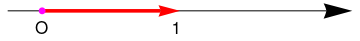
Choosing a Cartesian coordinate system for a one-dimensional space—that is, for a straight line—involves identification of a point O of the line (the origin), a unit of length, and an orientation for the line. An orientation chooses which of the two half-lines determined by O is the positive and which is negative; we then say that the line "is oriented" (or "points") from the negative half towards the positive half. Then each point P of the line can be specified by its distance from O, taken with a + or − sign depending on which half-line contains P. It is a custom to choose orientation from left to right following habits to write in all European languages.
A line with a chosen Cartesian system is called a number line, denoted by ℝ in mathematics. Every real number has a unique location on the line. Conversely, every point on the line can be interpreted as a number in an ordered continuum such as the real numbers.
Example 1:
Suppose you want to measure energy of the system or its temperature (these two concepts are closely related).
Actually, we can only measure energy/temperature differences, not energies/temperatures themselves. The reason is that we can add any real number to our definition of energy or temperature without changing any of the physics. This means it doesn't make much sense to ask what the energy of a system is---we can answer this question only after picking an arbitrary convention about what counts as "zero energy". What makes more sense is to talk about the difference between the energy of a system in one state and the energy of that system in some other state.
On a line, we choose a starting point that we call the origin and with some unit length we can identity energy or temperature values. Similar approach is valid in other physical problems.
In electric circuit, we can only measure voltage differences, not voltages themselves. The reason is that we can add any real number to our definition of the electromagnetic potential without changing any of the physics. In practical work with electrical circuits, we usually say the electromagnetic potential of the ground is zero. But this is an arbitrary choice.
Our next example is the set of real numbers ℝ that is a vector space over the set of scalars ℝ. Considering this set as a vector space, we denote it as ℝ¹. Similar conclusion is true for the field of rational numbers ℚ.
Example 2:
Let \( \displaystyle \texttt{D} = {\text d}/{\text d}x \) be the differential operator. Its null-space consists of all solutions of the differential equation
\[
\texttt{D}\, f = 0 \qquad \iff \qquad f' = 0 .
\]
So the null-space is a vector space of all real constants, that is, ℝ¹.
Vectors on the Plane
Although we claim to be 3-dimensional beings, much of our mathematical lives has been lived in the plane. Actual physical representations of planes are everywhere, from the screen of your laptop and sheet of paper on which
these words are printed, to the board on which your teacher writes, to the floor beneath your feet. Mathematically, the plane consists of points that have no dimensions (but pixels on your screen have).
There has been something missing from our good times in the plane however, and
what is missing is arithmetic. The notion of adding points may seem a bit odd because addition is for numbers, not points. However, addition is legitimate for vectors.
Most likely, you are familiar with (free) vectors on the plane that can be moved without changing their direction and magnitude.
It is a custom to identify vectors with arrows (geometric objects). The tail of
the arrow is called the initial point of the vector and the
tip the terminal point. To emphasis this approach, an arrow
is placed above the initial and terminal points, for example, the notation
\( {\bf v} = \vec{AB} \) tells us that A is
the starting point of the vector v and its terminal point is
B. In this tutorial (as in most science papers and textbooks), we will
denote vectors in boldface type applied to lower case letters such as
v, u, or x.
Any two vectors x and y can be added in "tail-to-head" manner; that is, either
x or y may be applied to any point and then another vector is applied to the
endpoint of the first. If this is done, the endpoint of the latter is the endpoint of their sum, which is denoted
by x + y. Besides the operation of vector addition there is another natural
operation that can be performed on vectors---multiplication by a scalar that are often taken to be real numbers.
When a vector is multiplied by a real number k, its magnitude is multiplied by |k| and its direction
remains the same when k is positive and the opposite direction when k is negative. Such vector is
denoted by kx.
These two sets, points and vectors, can be only identified with each other when a Cartesian system of coordinated is imposed on the plane. This requires choosing the origin, two perpendicular lines with orientation, and units in order to convert these lines into axes. Upon coordinization of the plane, we can identify its points (denoted geometrically by dots) with ordered pairs of numbers, known as coordinates. This allows us to establish one-to-one correspondence between these three sets: vectors, points on the plane, and ordered pairs of real numbers, denoted by ℝ².
The invention of Cartesian coordinates in 1649 by René Descartes (Latinized name: Cartesius) revolutionized mathematics by providing the first systematic link between Euclidean geometry and algebra.
With this correspondence, we can define addition between their elements of these three sets based on known rules for vectors:
Also, we can define multiplication by real numbers as
\[
k {\bf u} = k \left( u_1 , u_2 \right) = \left( k\,u_1 , k\,u_2 \right) .
\]
Vectors can be described also algebraically. Historically, the first vectors were Euclidean vectors that can be
expanded through standard basic vectors that are used as coordinates. Then any vector can be uniquely represented
by a sequence of scalars called coordinates or components. The set of such ordered n-tuples is denoted by 𝔽n, where set of scalars 𝔽 is usually one of the following three fields: either set of rational numbers ℚ or set of real numbers ℝ or set of complex numbers ℂ.
Motivated by these two approaches, we
present the general definition of vectors.
Vectors in ℝ²
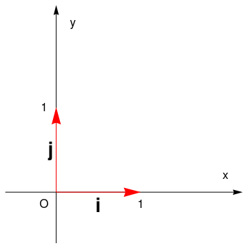
A Cartesian coordinate system in two dimensions (also called a rectangular coordinate system or an orthogonal coordinate system) is defined by an ordered pair of perpendicular lines (axes), a single unit of length for both axes, and an orientation for each axis. The point where the axes meet is taken as the origin for both, thus turning each axis into a number line. For any point P on the plane, a line is drawn through P perpendicular to each axis, and the position where it meets the axis is interpreted as a number. The two numbers, in that chosen order, are the Cartesian coordinates of P. The reverse construction allows one to determine the point P given its coordinates.
The coordinates are usually written as two numbers in parentheses, in that order, separated by a comma, as in (1, 2). Thus, the origin has coordinates (0, 0), and the points on the positive half-axes, one unit away from the origin, have coordinates (1, 0) and (0, 1). They are usually denoted by i and j, respectively.
In mathematics, physics, and engineering, the first axis is usually defined or depicted as horizontal and oriented to the right, called abscissa, and the second axis is vertical and oriented upwards; it is referred to as ordinate. (However, in some engineering problems and computer graphics contexts, the ordinate axis may be oriented downwards---navy prefers downwards.) The origin is often labeled O, and the two coordinates are often denoted by the letters X and Y, or x and y. The axes may then be referred to as the X-axis and Y-axis. The choices of letters come from the original convention, which is to use the latter part of the alphabet to indicate unknown values. The first part of the alphabet was used to designate known values.
We are accustomed to visualizing an ordered pair as a point in the plane and denoting it geometrically by a dot as shown in figure above. Physicists have found another very useful geometric interpretation of such pairs in their consideration of forces acting on a body. The motion in response to a force depends on the direction in which the force is exerted. It is natural to represent a force by an arrow, pointing in the direction in which the force is acting, and with the length of the arrow representing the magnitude of the force. Such an arrow is a force vector.
Vectors in ℝ³
To coordinatize space, we choose three mutually perpendicular lines as coordinate axes through a point that we call the origin, and label 0.
We also need to choose a
single unit of length for all three axes. As in the two-dimensional case, each axis becomes a number line. For any point P of space, one considers a hyperplane through P perpendicular to each coordinate axis, and interprets the point where that hyperplane cuts the axis as a number. The Cartesian coordinates of P are those three numbers, in the chosen order. The reverse construction determines the point P given its three coordinates.
Alternatively, each coordinate of a point P can be taken as the distance from P to the hyperplane defined by the other two axes, with the sign determined by the orientation of the corresponding axis.
Each pair of axes defines a coordinate hyperplane. These hyperplanes divide space into eight octants.
Example 4:
Although the process followed by the human brain in perceiving and interpreting color is a physiopsychological phenomenon that is not fully understood, the physical nature of color can be expressed on a formal basis supported by experimental and theoretical results.
In 1666, Sir Isaac Newton discovered that when a beam of sunlight passes through a glass prism, the emerging beam of light is not white but consists instead of continuous spectrum of colors ranging from violet at one end to red at the other. The color spectrum may be divided into six broad regions: violet, blue, green, yellow, orange, and red. When viewed in full color, no color in the spectrum ends abruptly, but rather each color blends smoothly into the next.
Characterization of light is central to the science of color. Chromatic light spans the electromagnetic spectrum from approximately 400 to 700 nm. Three basic quantities are used to describe the quantity of a chromatic light source: radiance, luminance, and brightness. Radiance is the total amount of energy that flows from the light source and it is usually measured in watt (W). Luminance, measured in lumens (lm), gives a measure of the amount of energy an observer perceives from alight source. Finally, brightness is a subjective descriptor that is practically impossible to measure. It embodies the achromatic (void of color) notion of intensity and is one of the key factors in the describing color sensation.
Due to absorption characteristics of the human eye, colors are seen as variable combinations of the so-called primary colors red (R), green (G), and blue (B). For the purpose of standardization, the CIE (Commission Internationale de l'Eclairage---the International Commission on Illumination) designated in 1931 the following specific wavelength values to the three primary colors: blue = 435.8 nm, green = 546.1 nm, and red = 700 nm.
Contemporal laptops, computer screens, and TV utilize "flat panel" digital technologies , such as liquid crystal displays (LCDs) and plasma devices. The amounts of red, green, and blue needed to form any particular color are called the tristimulus values, and are denoted, R, G, and B, respectively; they varies from 0 to 28 −1 = 255. A color is then specified by its trichromatic coefficients, defined as
\[
x = \frac{R}{R+G+B} , \qquad y = \frac{G}{R+G+B} , \qquad z = \frac{B}{R+G+B}
\]
In the RGB model, each color appears in its primary spectral components of red, green, and blue. This model is based on a rectangular coordinate system. The color subspace of interest is the cube, in which RGB primary values are at three corners; the secondary colors cyan, magenta, and yellow are at three other corners; black is at the origin; and white is at the corner farhest from the origin. In this model, the gray scale (points of equal RGB values) extends from black to white along the line joining these two points. The different colors in this model are points on or inside the cube, and are defined by vectors extending from the origin. For convenience, the assumption is that all color values have been normalized so that the cube is of unit length. One way to do this is to identify the primary colors with the vectors in ℝ³:
Similarly, we can define the Cartesian products of complex numbers ℂn or rational numbers ℚn.
Any two vectors x and y can be added in "tail-to-head" manner; that is, either
x or y may be applied to any point and then another vector is applied to the
endpoint of the first. If this is done, the endpoint of the latter is the endpoint of their sum, which is denoted
by x + y. Besides the operation of vector addition there is another natural
operation that can be performed on vectors---multiplication by a scalar that are often taken to be real numbers.
When a vector is multiplied by a real number k, its magnitude is multiplied by |k| and its direction
remains the same when k is positive and the opposite direction when k is negative. Such vector is
denoted by kx.
A vector spaceV over set of either real numbers or complex numbers is a set of elements,
called vectors, together with two operations that satisfy the eight axioms listed below.
1. The first operation is an inner operation that assigns to any two vectors x and y
a third vector which is commonly written as x + y and called the sum of these two
vectors.
2. The second operation, is an outer operation that assigns to any scalar k and vector x another vector,
denoted by kx.
Commutativity of addition: \( ({\bf v} + {\bf u}) = {\bf u} + {\bf v} \)
for \( ({\bf v} , {\bf u}) \in V . \)
Identity element of addition: there exists an element \( ({\bf 0} \in V , \) called
the zero vector, such that \( {\bf v} +{\bf 0}) = {\bf v} \) for every vector from V.
Inverse elements of addition: for every vector v, there exists an element
\( -{\bf v} \in V , \) called the additive inverse of v, such that
\( {\bf v} + (-{\bf v}) = {\bf 0} . \)
Compatibility of scalar multiplication with field multiplication: \( a(b{\bf v}) = (ab){\bf v} \)
for any scalars a and b and arbitrary vector v.
Identity element of scalar multiplication: \( 1{\bf v} = {\bf v} , \) where 1
denotes the multiplicative identity.
Distributivity of scalar multiplication with respect to vector addition: \( k\left( {\bf v} +
{\bf u}\right) = k{\bf v} + k{\bf u} \) for any scalar k and arbitrary vectors v and u.
Distributivity of scalar multiplication with respect to field addition: \( \left( a+b \right)
{\bf v} = a\,{\bf v} + b\,{\bf v} \) for any two scalars a and b and arbitrary vector v.
■
Addition of vectors
For two given vectors a and b, their sum a+b is determined as follows. We translate the vector b until its tail coincides with the head of a. (Recall such translation does not change a vector.) Then, the directed line segment from the tail of a to the head of b is the vector a+b.
Addition of two vectors
Before we define subtraction, we need to characterize the opposite of a vector, −a. The vector −a is the vector with the same magnitude as a but that is pointed in the opposite direction.
Vector opposite to the given vector
Now we define subtraction as addition with the opposite of a vector:
Subtraction of vectors
The addition/subtraction operation satisfies ordinary properties:
a + b = b + a (commutative law);
Commutative law
(a + b) + c = a + (b + c) (associative law);
There is a vector 0 such that b + 0 = b (additive identity);
For any vector a, there is a vector −a such that a + (−a) = 0 (Additive inverse).
Scalar multiplication
Given a vector a and a real number (scalar) λ, we can form the vector λa as follows. If λ is positive, then λa is the vector whose direction is the same as the direction of a and whose length is λ times the length of a. In this case, multiplication by λ simply stretches (if λ>1) or compresses (if 0<λ<1) the vector a.
If, on the other hand, λ is negative, then we have to take the opposite of a before stretching or compressing it. In other words, the vector λa points in the opposite direction of a, and the length of λa is |λ| times the length of a. No matter the sign of λ, we observe that the magnitude of λa is |λ| times the magnitude of a: ∥λa∥ = |λ| ∥a∥. Scalar multiplications satisfies many of the same properties as the usual multiplication.
λ(a + b) = λa + λb (distributive law, for vectors)
(λ + β)a = λa + βb (distributive law for scalars);
1·a = a;
(−1)·a = −a;
0·a = 0.
In the last formula, the zero on the left is the scalar 0, while the zero on the right is the vector 0, which is the unique vector whose length is zero.
If a = λb for some scalar λ, then we say that the vectors a and b are parallel. If λ is negative, then it is a common slang to say that a and b are anti-parallel, but we will not use that language.
Generalizing well-known examples of vectors (velocity and force) in physics and engineering, mathematicians introduced abstract object called vectors. So vectors are objects that can be added/subtracted and multiplied by scalars. These two operations (internal addition and external scalar multiplication) are assumed to satisfy natural conditions described above.
A set of vectors is said to form a vector space (also called a linear space), if any vectors from it can be added/subtracted and multiplied by scalars, subject to regular properties of addition and multiplication. Wind, for example, has both a speed and a direction and,
hence, is conveniently expressed as a vector. The same can be said of moving objects, momentum, forces, electromagnetic fields, and weight.
(Weight is the force produced by the acceleration of gravity acting on a mass.)
The first thing we need to know is how to define a vector so it
will be clear
to everyone. Today more than ever, information technologies are an integral
part of our everyday lives. That is why we need a tool to model vectors on
computers. One of the common ways to do this is to introduce a system of
coordinates, either Cartesian or any other.
In engineering, we
traditionally use the
Cartesian
coordinate system that specifies any point with a string of digits. Each
coordinate measures a distance from a point to its perpendicular projections
onto the mutually perpendicular hyperplanes.
Let us start with our familiar three dimensional space in which the
Cartesian coordinate system consists of an ordered triplet of lines (the axes)
that go through a common point (the origin), and are pair-wise perpendicular;
it also includes an orientation for each axis and a single unit of length for
all three axes. Every point is
assigned distances to three mutually perpendicular planes, called coordinate planes (such that the pair x and y axes define the z-plane, x and z axes define the y-plane, etc.).
The reverse construction determines the point given its three coordinates.
Each pair of axes defines a coordinate plane. These planes divide space into
eight trihedra, called
octants. The coordinates are usually written as three numbers (or algebraic
formulas) surrounded by parentheses or brackets and separated by commas, as in
(-2.1,0.5,7) or [-2.1,0.5,7]. Thus, the origin has coordinates (0,0,0), and the unit points
on the three axes are (1,0,0), (0,1,0), and (0,0,1).
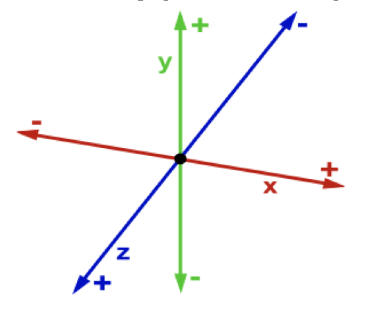
Axes for a 3D Space
There are no universal names for the coordinates in the three axes. However,
the horizontal axis is traditionally called abscissa borrowed from New
Latin (short for linear abscissa, literally, "cut-off line"), and usually
denoted by x. The next axis is called ordinate, which came from
New Latin (linear), literally, line applied in an orderly manner; we will
usually label it by y. The last axis is called applicate and
usually denoted by z. Correspondingly,
the unit vectors are denoted by i
(abscissa), j (ordinate), and k
(applicate), called the basis. Once rectangular coordinates are set up, any vector can be expanded through these unit
vectors. In the three dimensional case, every vector can be expanded as \( {\bf v} = v_1 {\bf i} + v_2 {\bf j} + v_3 {\bf k} ,\) where \( v_1, v_2 , v_3 \) are called the coordinates of the vector v. Coordinates are always specified relative to an ordered basis. When a basis has been chosen, a vector can be expanded with respect to the basis vectors and it can be identified with an ordered n-tuple of n real (or complex) numbers or coordinates. The set of all real (or complex) ordered numbers is denoted by ℝn (or ℂn).
In general, a vector in infinite dimensional space is identified by an infinite sequence
of numbers. Finite dimensional coordinate vectors can be represented by
either a column vector (which is usually the case) or a row vector. We will
denote column-vectors by lower case letters in bold font, and row-vectors by
lower case letters with a superimposed arrow. Because of the way the Wolfram Language uses lists to represent vectors, Mathematica does not distinguish
column vectors from row vectors, unless the user specifies
which one is defined. One can define vectors using Mathematica
commands: List, Table, Array, or curly brackets.
In applications, people deal with a variety of quantities that are used to describe the physical world. Examples of
such quantities include distance, displacement, speed, velocity, acceleration, force, mass, momentum, energy, work,
power, etc. All these quantities can by divided into two categories -- vectors and scalars. A vector quantity is a
quantity that is fully described by both magnitude and direction. On the other hand, a scalar quantity is a quantity
that is fully described by its magnitude.
In mathematics, physics, and engineering, a Euclidean vector
(simply a vector) is a geometric object that has magnitude (or length) and
direction. Many familiar physical notions, such as forces, velocities, and
accelerations, involve both magnitude (the amount of the force, velocity, or
acceleration) and a direction. In most physical situations involving vectors,
only the magnitude and direction of the vector are significant; consequently,
we regard vectors with the same length and direction as being equal
irrespective to their positions.