Let us remind some information that is related to the topic of this section.
For any two sets A and B, their Cartesian product consists of all ordered pairs (𝑎, b) such that 𝑎 ∈ A and b ∈ B,
\[
A \times B = \left\{ (a,b)\,:\ a \in A, \quad b\in B \right\} .
\]
If sets A and B carry some algebraic structure, as in our case, they are vector spaces, then we can define a suitable structure on the product set as well. So, direct product is like Cartesian product, but with
some additional structure. In our case, we equip it with addition operation
\[
k \left( a , b \right) = \left( k\,a , k\,b \right) , \qquad k \in \mathbb{F}.
\]
Here 𝔽 is a field of scalars (either ℚ, rational numbers, or ℝ, real numbers, or ℂ, complex numbers). It is a custom to denote the direct product of two or more scalar fields as 𝔽² = 𝔽×𝔽 or, more generally, 𝔽n.
Theorem 1:
Let X1, X2, … , Xn be finite-dimensional vector spaces over the same field. Then
X1×X2× ⋯ ×Xn is finite-dimensional and
\[
\dim \left( X_1 \times X_2 \times \cdots \times X_n \right) = \dim X_1 + \dim X_2 + \cdots + \dim X_n .
\]
Choose a basis of each Xj, j = 1, 2, … , n. For each basis vector of each Xj, consider
the element of X1×X2× ⋯ ×Xn that equals the basis vector in the j-th slot and
0 in the other slots. The list of all such vectors is linearly independent and
spans X1×X2× ⋯ ×Xn. Thu,s it is a basis of X1×X2× ⋯ ×Xn. The length of this
basis is dimX1 + dimX2 + ⋯ + dimXn, as desired.
Example 1:
Elements of ℝ³ × ℝ² are lists
\[
\left( \left( x_1 , x_2 , x_3 \right) , \left( y_1 , y_2 \right) \right) , \qquad x_1, x_2 , x_3 , y_1 , y_2 \in \mathbb{R} .
\]
On the other hand, elements of ℝ⁵ are lists (x₁,
x₂, x₃, x₄, x₅), where every component is a real number.
Although these look almost the same, they are not the same kind of objects.
Elements of ℝ³ × ℝ² are lists of length 2 (with the first item itself a list of
length 3 and the second item a list of length 2), and elements of ℝ⁵ are lists
of length 5. Thus, ℝ³ × ℝ² does not equal to ℝ⁵.
The linear map that takes a vector ((x₁, x₂, x₃), (y₁, y₂)) ∈ ℝ³ × ℝ² to (x₁, x₂, x₃, (y₁, y ₂) ∈ ℝ⁵ is clearly an isomorphism of ℝ³× ℝ² onto ℝ⁵.
Hence, these two vector spaces are isomorphic.
In this case, the isomorphism is so natural that we should think of it as a
relabeling. Some people would even informally say that ℝ³ × ℝ² equalsℝ⁵, which is not technically correct but which captures the spirit of identification
via relabeling.
End of Example 1
■
It turns out that a direct product of two vector spaces can be considered as a sum. In this case, it is called the direct sum and denoted as A⊕B. For a finite dimensional vector spaces, the direct product and direct sum are identical constructions (mathematically speaking, they are isomorphic), and these terms are often used interchangeably.
There are two reasons to use the sum of two vector spaces. One of them is the way to build new vector spaces from old
ones. Another reason is to decompose the known vector space into sum of two (smaller) spaces. This leads to several equivalent definitions of corresponding sums that are referred to as the direct sums.
Sum of Two Subspaces
The following definition considers only sum of two subsets of a vector space. However, it is crystal clear how to expand this definition for arbitrary finite number of subsets.
Let A and B be nonempty subsets of a vector space V. The sum of A and B,
denoted A + B, is the set of all possible sums of elements from both subsets:
\( A+B = \left\{ a+b \, : \, a\in A, \ b\in B \right\} . \)
The sum of two subspaces U and W is the subspace of V generated by U and W. If A is a set of generators of
U, B a set of generators of W, then A U B generates U + W. If u ∈ U, w ∈ W,
and x ∈ U ∩ W, then
shows that the elements of the sum U + W. may have several representations as sums. Uniqueness of decomposition requires U ∩ W = {0}.
Example 2:
Let V = ℝ³ be the usual real 3-dimensional space, X the horizontal plane
defined by z = 0, and Y the vertical plane defined by x = 0. Then each vector
of ℝ³ has a decomposition
\[
\begin{bmatrix} x \\ y \\ z \end{bmatrix} = \underbrace{ \begin{bmatrix} x \\ y+a \\ 0 \end{bmatrix}}_{\in X} + \underbrace{\begin{bmatrix} 0 \\ y-a \\ z \end{bmatrix} }_{\in Y}
\]
for arbitrary 𝑎 ∈ ℝ. Therefore, the decomposition X + Y = ℝ³ is valid for arbitrary scalar 𝑎 with components in X and respectively in Y. Not that
\[
\begin{bmatrix} 0 \\ a \\ 0 \end{bmatrix} \in X \cap Y , \qquad a \in \mathbb{R}.
\]
Theorem 2:
Let X and Y be two subspaces of a vector space V over scalar field 𝔽.
If α is a basis of X and β a basis of Y,
then α U β is a basis of X + Y.
Any vector v ∈ X + Y is a sum of two vectors
\[
{\bf v} = {\bf x} + {\bf y} , \qquad {\bf x} \in X, \quad {\bf y} \in Y .
\]
Each of the vectors x and y can be expanded via elements from basis α (correspondingly β) as
\[
{\bf x} = a_1 {\bf e}_1 + a_2 {\bf e}_2 + \cdots + c_k {\bf e}_k , \qquad {\bf y} = b_1 {\bf w}_1 + w_2 {\bf w}_2 + \cdots + b_n {\bf w}_n ,
\]
where ei and wj are elements of bases α and β, respectively. This allows us to expand arbitrary vector v as
\[
{\bf v} = a_1 {\bf e}_1 + a_2 {\bf e}_2 + \cdots + c_k {\bf e}_k + b_1 {\bf w}_1 + w_2 {\bf w}_2 + \cdots + b_n {\bf w}_n \in X+Y.
\]
Of course, the expansion of v is not unique because the union α ∪ β may contain linearly dependent elements.
Theorem 3:
If X and Y are subspaces of a vector space V, then
\[
\dim \left( X + Y \right) = \dim \left( X \right) + \dim \left( Y \right) - \dim \left( X \cap Y \right) .
\]
Let S be a basis of X∩Y. If X ∩ Y is the zero space then S = 𝔽. We extend S = { s1, s2, … , sr } to a basis α = { s1, s2, … , sr, v1, … , vk } of X. Similarly, basis β of Y can be written as β = { s1, s2, … , sr, u1, … , un }. Then dim(X∩Y) = r and dim(X) = r + k, dim(Y) = r + n.
Upon this construction, we get the basis of X + Y to be
B = { s1, s2, … , sr, v1, … , vk, u1, … , un }. So the dimension of the sum is
\[
r + k + n = \left( r + k \right) + \left( r + n \right) - r .
\]
Example 3:
We consider three hyperspaces in ℝ³:
\[
X = \left\{ \begin{bmatrix} 0 \\ y \\ z \end{bmatrix} : \ y,z \in \mathbb{R} \right\} , \quad Y = \left\{ \begin{bmatrix} x \\ 0 \\ z \end{bmatrix} : \ x,z \in \mathbb{R} \right\} , \quad Z = \left\{ \begin{bmatrix} x \\ y \\ 0 \end{bmatrix} : \ x,y \in \mathbb{R} \right\} .
\]
Their intersections are
\[
X\cap Y = \left\{ \begin{bmatrix} 0 \\ 0 \\ z \end{bmatrix} : \ z \in \mathbb{R} \right\} , \quad Y\cap Z = \left\{ \begin{bmatrix} x \\ 0 \\ 0 \end{bmatrix} : \ x \in \mathbb{R} \right\} , \quad X\cap Z = \left\{ \begin{bmatrix} 0 \\ y \\ 0 \end{bmatrix} : \ y \in \mathbb{R} \right\} .
\]
Obviously, X + Y + Z = ℝ³, so dim(X + Y + Z) = 3. Their pairwise intersections are all one-dimensional, and subspaces X, Y, and Z are two-dimensional:
\[
\dim \left( X \cap Y \right) = \dim \left( X \cap Z \right) = \dim \left( Y \cap Z \right) = 1,
\]
and
\[
\dim \left( X \right) = \dim \left( Y \right) = \dim \left( Z \right) = 2.
\]
Hence, we verify formula (1) that follows:
\begin{align*}
\dim \left( X + Y +Z \right) &= \sim \left( \mathbb{R}^3 \right) = 3,
\\
\dim \left( X \right) &= \dim \left( Y \right) = \dim \left( Z \right) = 2,
\\
\dim \left( X \cap Y \right) &= \dim \left( X \cap Z \right) = \dim \left( Y \cap Z \right) = 1,
\end{align*}
which gives
\[
3 = 2 + 2 + 2 - 1 -1 -1 .
\]
End of Example 2
■
Theorem 3 can be expanded for three and more subspaces using principle of inclusion and exclusion. In particular, for three subspaces X, Y, and Z of a vector space V, we have
\begin{equation} \label{EqDirect.1}
\begin{split}
\dim \left( X + Y + Z \right) &= \dim \left( X \right) + \dim \left( Y \right) + \dim \left( Z \right)
\\
&\quad - \dim \left( X \cap Y \right) - \dim \left( X \cap Z \right) - \dim \left( Y \cap Z \right)
\\
&\quad + \dim \left( X \cap Y \cap Z \right) . \end{split}
\end{equation}
A complement to a subspace X of a vector space V is another subspace Y such that X ∩ Y = {0}. Two subspaces X and Y are said to be supplement of each other, when X + Y = V and X ∩ Y = {0}.
Theorem 4:
Every subspace X of a finite dimensional vector space V has a complement in V.
Since X is a subspace of a finite dimensional vector space V, it has a basis α = { e1, e2, … , ek } that can be extended to the basis β = { e1, e2, … , ek, u1, … , um } of vector space V. Using set of vectors S = { u1, … , um } as a generator, we build a subspace Y as a span of S, so Y = span(S). Then Y is a complementary subspace of X because X ∩ Y = {0}.
Example 4:
Let us consider a two-dimensional plane of solutions to the linear equation
\[
x + 2\,y - 3\,z = 0 .
\tag{4.1}
\]
From this equation, we find x = −2y + 3z, which we use to represent arbitrary solution as
\[
{\bf v} = \begin{bmatrix} x \\ y \\ z \end{bmatrix} = \begin{bmatrix} -2y+3z \\ y \\ z \end{bmatrix} = y \begin{bmatrix} -2 \\ 1 \\ 0 \end{bmatrix} + z \begin{bmatrix} 3 \\ 0 \\ 1 \end{bmatrix} .
\]
Therefore, the solution set X of Eq.(4.1) is spanned on two vectors
We know that the solution set X is a two-dimensional vector space generated by vectors (4.2). A line Y spanned on the vector u = (𝑎, b, c) does not belong to subspace X if and only if the determinant of the matrix
\[
\det \begin{bmatrix} \phantom{-}a & b & c \\ -2 & 1 & 0 \\ \phantom{-}3 & 0 & 1 \end{bmatrix} = a + 2b -3c \ne 0
\tag{4.3}
\]
For example, if we choose 𝑎 = c = 0, b = 1, and take Y to be abscissa (spanned on (0,1,0) vector space), then X⊕Y = ℝ³.
End of Example 3
■
Direct Sums of Vector Spaces
Since we consider linear
transformations between vector spaces, these sums lead to representations of these linear maps and
corresponding matrices into forms that reflect these sums. In many very important situations, we start with a vector
space V and can identify subspaces “internally” from which the whole space V can be built up using the
construction of sums. However, the most fruitful results we obtain for a special sum, called the direct sum.
Let X and Y be subspaces of a vector space V. If every vector v ∈ V can be uniquely expressed as the sum v = x + y, where x ∈ X and y ∈ Y, then V is said to
be the direct sum of X and Y, and we write V = X⊕Y.
In general, V is the direct sum of subspaces X1,
X2, … , Xn, denoted V =
X1⊕X2⊕⋯⊕Xn, if every vector v from V can be decomposed in a unique way as
\[
{\bf v} = {\bf x}_1 + {\bf x}_2 + \cdots + {\bf x}_n, \qquad {\bf x}_i \in X_i , \quad i = 1,2,\ldots , n.
\]
The statement X⊕Y is meaningless unless both spaces X and Y are subspaces of one larger vector space.
Lemma 1:
Let V be a vector space that is a direct sum of two subspaces: V = X⊕Y.
Whenever 0 = x + y with x∈X, y∈Y, then x = y = 0.
Informally, when we say V is the direct sum of the subspaces X and Y, we are saying that each vector of V can always be expressed as the sum of a vector from X and a vector from Y, and this expression can only be accomplished in one way (i.e., uniquely).
Theorem 5:
Suppose that X and Y are subspaces of a vector space V so that V = X + Y. Then V = X⊕Y if and only if X ∩ Y = {0}.
Suppose there exists a nonzero vector u &isinl X ∩ Y. Then u = u + 0, with u ∈ X, 0 ∈ Y, and u = 0 + u, with 0 ∈ X, u ∈ Y. This contradicts our uniqueness
assumption.
Conversely, suppose that X ∩ Y = {0}, but we have two distinct expansions v = a + b = c + d, with
a, c ∈ X and b, d ∈ Y. Then a − c = b − d. Then the LHS a − c is in X but the RHS b − d belongs to Y. Therefore, this vector is in X ∩ Y, which must be {0}. So a = c and b = d.
Example 5:
The vector space of square matrices ℝn,n over the field of real numbers can be decomposed into direct sum ℝn,n = S ⊕ A of symmetric matrices A = AT and anti-symmetric matrices A = −AT, respectively:
\[
{\bf A} = \frac{1}{2} \left( {\bf A} + {\bf A}^{\mathrm{T}} \right) + \frac{1}{2} \left( {\bf A} - {\bf A}^{\mathrm{T}} \right) .
\]
As an illustrative example, let us consider a square matrix
A = {{1, 2, 3}, {4, 5, 6}, {7, 8, 9}};
As = (A + Transpose[A])/2
{{1, 3, 5}, {3, 5, 7}, {5, 7, 9}}
Aa = (A - Transpose[A])/2
{{0, -1, -2}, {1, 0, -1}, {2, 1, 0}}
End of Example 5
■
Since any vector subspace and its complement form a direct sum, we get the following result.
Corollary 1:
Suppose that X is a subspace of the vector space V. Then there exists a subspace Y of V such that V = X⊕Y.
The direct sum mimic very closely the definition of bases. Just like bases must span the
entire vector space, so too must subspaces in a direct sum, and just like bases
must be “small enough” that they are linearly independent, subspaces in a direct
sum must be “small enough” that they only contain the zero vector in common.
Another useful equivalent formulation of direct sums can be defined using a linear transformation. If X1, … , Xn are subs[aces of a vector space V, then we can define a linear function
The image of Γ is by definition the subspace of the vector space X1 + X2 + ⋯ + Xn.
Theorem 6:
The sum of vectors subspaces X1 + X2 + ⋯ + Xn is a direct sum if and only if linear transformation (2) is injective.
The linear map Γ is injective if and only if the only way to write 0 as a sum x1 + x2 + ⋯ + xn, where each xj is in Xj, is by taking each xj equal to 0. But this is exactly the requirement of the sum to be direct.
Example 6:
Consider the Cartesian plane \( \mathbb{R}^2 , \)
when every element is represented by an ordered pair v = (x,y). This vector has a unique decomposition
\( {\bf v} = (x,y) = {\bf v}_1 + {\bf v}_2 = (x,0) + (0,y) , \) where vectors (x,0) and
(0,y) can be identified with a one-dimensional space \( \mathbb{R}^1 = \mathbb{R} . \)
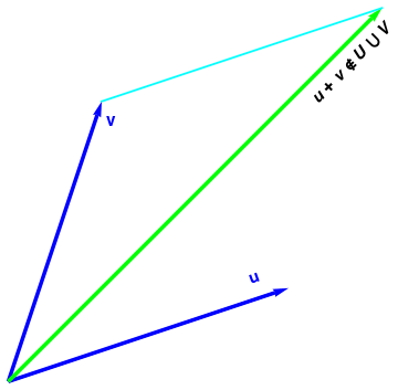
If we choose two arbitrary not parallel vectors u and v on the plane, then spans of these vectors generate two
vectors spaces that we denote by U and V, respectively. Therefore, U and V are two lines
containing vectors u and v, respectively. Their sum, \( U + V = \left\{ {\bf u} +{\bf v} \,: \
{\bf u} \in U, \ {\bf v} \in V \right\} \) is the whole plane \( \mathbb{R}^2 . \)
The union \( U \cup V \) of two subspaces is not necessarily a subspace.
End of Example 6
■
Theorem 7:
The sum of vectors subspaces X1 + X2 + ⋯ + Xn is a direct sum if and only if dimensions add up
\[
\dim \left( X_1 + X_2 + \cdots + X_n \right) = \dim X_1 + \dim X_2 + \cdots + \dim X_n .
\]
We prove Theorem 7 by induction. For two subspaces of a vector space V, we know from Theorem 3 that
\[
\dim \left( X + Y\right) = \dim X + \dim Y - \dim \left( X \cap Y \right) .
\tag{P7.1}
\]
For a direct sum of X⊕Y, we have from Theorem 5 that X∩Y = {0}. Hence, from Eq.(P7.1}, it follows that
\[
\dim \left( X \oplus Y\right) = \dim \left( X + Y\right) = \dim X + \dim Y .
\tag{P7.2}
\]
Now suppose that Theorem 7 is valid for arbitrary n terms:
\[
\dim \left( X_1 + \cdots + X_n \right) = \dim \left( X_1 \oplus \cdots \oplus X_n \right) = \dim X_1 + \cdots + \dim X_n .
\tag{P7.3}
\]
Then for n + 1 terms, we obtain from Eq.(P7.1) that
\[
\dim \left( X_1 + \cdots + X_n + X_{n+1} \right) = \dim \left( U + X_n \right) = \dim U + \dim X_{n+1} ,
\]
where U = X1 + ⋯ + Xn. Since for sum U of n terms formula (P7.3) is valid accoreding to induction assumption. we conclude that Theorem 7 is valid for n + 1 terms.
Example 7:
Let E denote the set of all polynomials of even powers:
\( E = \left\{ a_n t^{2n} + a_{n-1} t^{2n-2} + \cdots + a_0 \right\} , \) and O
be the set of all polynomials of odd powers: \( O = \left\{ a_n t^{2n+1} + a_{n-1} t^{2n-1} + \cdots + a_0 t \right\} . \)
Then the set of all polynomials P is the direct sum of these sets: \( P = O\oplus E . \)
It is easy to see that any polynomial (or function) can be uniquely decomposed into direct sum of even and odd counterparts:
Theorem 8:
Suppose X and Y are subspaces of the vector space V that form the direct sum V = X⊕Y. If R is a linearly independent subset of X and S is a linearly independent subset of Y, then their union R∪S is a linearly independent subset of V. and
Let R = { r1, r2, … , rs } and S = { s1, s2, … , sr }. Their union R∪S is a linearly dependent if and only if there exists a set of scalars (not all equal to zero) such that
\\begin{align*}
{\bf 0} &= \alpha_1 {\bf r}_1 + \cdots + \alpha_s {\bf r}_s + \beta_1 {\bf s}_1 + \cdots + \beta_r {\bf s}_r .
\\
&= {\bf u} + [\bf w} ,
\end{align*}
where &alpha1r1 + ⋯ +&alphasrs = u ∈ X and
&beta1s1 + ⋯ +&betarsr = w ∈ Y.
Now applying Lemma 1, the linear independence of R and S (individually) yields
\[
\alpha_1 + \cdots + \alpha_ s = 0 , \qquad \beta_1 + \cdots + \beta_r = 0.
\]
Direct Sums of Matrices
Suppose that an n-dimensional vector space V is the direct sum of two subspaces \( V = U\oplus W . \)
Let \( {\bf e}_1 , {\bf e}_2 , \ldots , {\bf e}_k \) be a basis of the linear subspace
U and let \( {\bf e}_{k+1} , {\bf e}_{k+2} , \ldots , {\bf e}_n \) be a basis of the linear subspace
W. Then \( {\bf e}_1 , {\bf e}_2 , \ldots , {\bf e}_n \) form a basis of the whole
linear space V. Any linear transformation written in this basis has a matrix representation:
Therefore, the block diagonal matrix A is the direct sum of two matrices of lower sizes.
Example 8:
Let us consider the set M of all real (or complex) m × n
matrices, and let \( U = \left\{ {\bf A} = \left[ a_{ij} \right] :\, a_{ij} =0 \ \mbox{ for } i > j\right\} \)
be the set of upper triangular matrices, and let
\( W = \left\{ {\bf A} = \left[ a_{ij} \right] :\, a_{ij} =0 \ \mbox{ for } i \le j\right\} \)
be the set of lower triangular matrices. Then \( M = U \oplus W . \) ■
Before formulating the Primary Decomposition Theorem, we need to recall some definitions and facts that were explained in other sections.
We remind that the minimal polynomial of a square matrix A (or corresponding linear transformation)
is the (unique) monic polynomial ψ(λ) of least degree that annihilates the matrix A, that is
ψ(A) = 0. The minimal polynomial\( \psi_u (\lambda ) \) of a
vector \( {\bf u} \in V \ \mbox{ or } \ {\bf u} \in \mathbb{R}^n \) relative to A is the
monic polynomial of least degree such that
\( \psi_u ({\bf A}) {\bf u} = {\bf 0} . \) It follows that \( \psi_u (\lambda ) \)
divides the minimal polynomial ψ(λ) of the matrix A. There exists a vector
\( {\bf u} \in V (\mathbb{R}^n ) \) such that
\( \psi_u (\lambda ) = \psi (\lambda ) . \) This result can be proved by representing
the minimal polynomial as the product of simple terms to each of which corresponds a subspace. Then the original vector
space (or \( \mathbb{R}^n \) ) is the direct sum of these subspaces.
A subspace U of a vector space V is said to be T-cyclic with respect to a linear transformation
\( T\,:\, V \to V \) if there exists a vector \( {\bf u} \in U \)
and a nonnegative integer r such that \( {\bf u}, T\,{\bf u} , \ldots , T^r {\bf u} \)
form a basis for U. Thus, for the vector u if the degree of the minimal polynomial
\( \psi_u (\lambda ) \) is k, then
\( {\bf u}, T\,{\bf u} , \ldots , T^{k-1} {\bf u} \) are linearly independent and the space
U is spanned by these k vectors is T-cyclic.
Theorem (Primary Decomposition Theorem): Let V be an
n-dimensional vector space (n is finite) and T is a linear transformation on V.
Then V is the direct sum of T-cyclic subspaces. ■
Let k be the degree of the minimal polynomial ψ(λ) of transformation T (or corresponding matrix
written is specified basis), and let u be a vector in V with
\( \psi_u (\lambda ) = \psi (\lambda ) . \) Then the space U spanned by
\( {\bf u}, T{\bf u} , \ldots , T^{k-1} {\bf u} \) is T-cyclic. We shall prove that if
\( U \ne V \quad (k \ne n), \) then there exists a T-invariant subspace W such
that \( V = U\oplus W . \) Clearly, by induction on the dimension, W will then be the
direct sum of T-cyclic subspaces and the proof is complete.
To show the existence of W enlarge the basis
\( {\bf e}_1 = {\bf u}, {\bf e}_2 = T{\bf u} , \ldots , {\bf e}_k = T^{k-1} {\bf u} \) of
U to a basis \( {\bf e}_1 , {\bf e}_2 , \ldots , {\bf e}_k , \ldots , {\bf e}_n \)
of V and let
\( {\bf e}_1^{\ast} , {\bf e}_2^{\ast} , \ldots , {\bf e}_k^{\ast} , \ldots , {\bf e}_n^{\ast} \)
be the dual basis in the dual space. Recall that the dual space consists of all linear forms on V or, equivalently,
of all functionals on V. To simplify notation, let z = ek*. Then
Consider the dual space U* spanned by
\( {\bf z}, T^{\ast} {\bf z} , \ldots , T^{\ast\, k-1} {\bf z} . \)
Since ψ(λ) is also the minimal polynomial of T*, the space U* is
T*-invariant. Now observe that if
\( U^{\ast} \cap U^{\perp} = \{ 0 \} \) and dim U* = k, then
\( V^{\ast} = U^{\ast} \oplus U^{\perp} , \) where U* and
\( U^{\perp} \) are T*-invariant (since dim \( U^{\perp} \) = n-k).
This in turn implies the desired decomposition \( V = U^{\perp\perp} \oplus U^{\ast\perp} = U \oplus W , \)
where \( U^{\perp\perp} = U \) and \( U^{\ast\perp} = W \)
are T-invariant.
Finally, we shall prove that \( U^{\ast} \cap U^{\perp} = \{ 0 \} \) and
dim U* = k simultaneously as follows. Suppose that
\( a_0 {\bf z} + a_1 T^{\ast} {\bf z} + \cdots + a_s T^{\ast s} {\bf z} \in U^{\perp} , \)
where \( a_s \ne 0 \) and \( 0 \le s \le k-1 . \) Then
This matrix has the characteristic polynomial \( \chi (\lambda ) = \left( \lambda -1 \right)^3 \)
while its minimal polynomial is \( \psi (\lambda ) = \left( \lambda -1 \right)^2 . \)
The matrix A has two linearly independent eigenvectors
Let U and V be one-dimensional subspaces generated by spans of vectors u and v, respectively.
The minimal polynomials of these vectors are the same:
\( \psi_u (\lambda ) = \psi_v (\lambda ) = \lambda -1 \) because
Each of these one-dimensional subspaces U and V are A-cyclic and they cannot form the direct sum of
\( \mathbb{R}^3 . \) We choose a vector \( {\bf z} = \left[ 7, -3, 1 \right]^{\mathrm T} , \)
which is perpendicular to each u and v. matrix A transfers z into the vector
\( {\bf A}\,{\bf z} = \left[ 125, 192, 60 \right]^{\mathrm T} , \) which is perpendicular to
neither u nor v. Next application of A yields