
Introduction to Linear Algebra
Systems of Linear Equations
- Introduction
- Linear Systems
- Vectors
- Linear combinations
- Matrices
- Planes in ℝ³
- Reduced Row-Echelon Form
- Equation A x = b
- Sensitivity of solutions
- Linear independence
- Plane transformations
- Space transformations
- Linear transformations
- Affine maps
- Exercises
- Answers
Matrix Algebra
- Introduction
- Manipulation of matrices
- Partitioned matrices
- Block matrices Matrix operators
- Determinants
- Cofactors
- Cramer's rule
- Equivalent matrices
- Elimination: A = L U
- PLU factorization
- Reflection
- Givens rotation
- Special matrices
- Exercises
- Answers
Vector Spaces
- Introduction
- Motivation
- Vector Spaces
- Bases
- Dimension
- Coordinate systems
- Change of basis
- Linear transformations
- Matrix transformations
- Compositions
- Isomorphisms
- Dual transformations
- Direct sums
- Quotient spaces
- Rank
- Solving A x = b
- Exercises
- Answers
Eigenvalues, Eigenvectors
- Introduction
- Characteristic polynomials
- Companion matrix
- Algebraic and geometric multiplicities
- Minimal polynomials
- Eigenspaces
- Where are eigenvalues?
- Eigenvalues of A B and B A
- Generalized eigenvectors
- Similarity
- Diagonalizability
- Self-adjoint operators
Euclidean Spaces
- Introduction
- Dot product
- Bilinear transformations
- Inner product
- Norm and distance
- Matrix norms
- Dual norms
- Dual transformations
- Orthogonality
- Gram--Schmidt Process
- Orthogonal sets
- Self-adjoint matrices
- Unitary matrices
- Projection operators
- QR-decomposition
- Least Square Approximation
- Quadratic forms
- Exercises
- Answers
Matrix Decompositions
- Introduction
- Symmetric matrices
- LU-decomposition
- Sylvester Formula
- Cholesky decomposition
- Schur decomposition
- Positive matrices
- Roots
- Polar factorization
- Spectral decomposition
- Singular values
- SVD <
- Pseudoinverse
- Exercises
- Answers
Applications
- GPS problem
- Poisson equation
- Graph theory
- Error correcting codes
- Electric circuits
- Markov chains
- Cryptography
- Wave-length transfer matrix
- Computer graphics
- Linear Programming
- Hill's determinant
- Fibonacci matrices
- Discrete dynamic systems
- Discrete Fourier transform
- Fast Fourier transform
- Curve fitting
Functions of Matrices
- Introduction
- Diagonalization
- Sylvester formula
- The Resolvent method
- Polynomial interpolation
- Positive matrices
- Roots <
- Pseudoinverse
- Exercises
- Answers
Miscellany
- Circles along curves
- TNB frames
- Tensors
- Tensors in ℝ³
- Tensors & Mechanics
- Differential forms
- Calculus
- Vector Representations
- Matrix Representations
- Change of Basis
- Orthonormal Diagonalization
- Generalized Inverse
Preliminaries
- Complex Number Operations
- Sets
- Polynomials
- Polynomials and Matrices
- Computer solves Systems of Linear Equations
- Location of Eigenvalues
- Power Method
- Iterative Method
- Similarity and Diagonalization
Glossary
Reference

This Book is licensed under Creative Commons Attribution-NonCommercial-NoDerivs 3.0 Unported License
Recall that in this tutorial we employ the notation 𝔽 for one of the following fields: either ℚ for rational numbers, or ℝ for real numbers, or ℂ for complex numbers. However, most examples involve field ℤ of integer numbers for historical reasons and to simplify exposition.
This section is divided into a number of subsections, links to which are:
Duality in matrix/vector multiplication
Elementary reduction operations
Geometric Interpretation
Note that the dot-product defines metric or distance only when field 𝔽 is real, but in case of complex numbers, it is just a linear combination of the products of the vector's components. Equation (1) presents a linear equation in standard form where constant term b is separated by sign "=" from the linear combination of vectors a = (𝑎₁, 𝑎₂, … , 𝑎n) and x = (x₁, x₂, … , xn). The standard form requires that every independent variable appears in the equation only once. Since we are going to modify the linear equation (1), it is convenient to assume that the order in which summation is performed remains the same in further manipulations; so you can choose any order of summation, but you have to be consistent.
The word "affine" is Latin-French meaning "related to" or "having affinity with." Below we illustrate a 2-dimensional affine subspace contained within a 3D space. This could be any plane that (a) need not pass through the origin; and (b) that fits within the larger dimension.
Using ParametricPlot3D, we start with 50 points, p = p₀ + 𝑎*v₁ + b*v₂, where 𝑎 and b are, each, a set of 50 parameters taking (for convenience) any real value between -2 and 2. p₀, v₁ and v₂ are fixed vectors in ℝ³. The graphic this produces looks like a random cluster of points contained in a 3D box.
p0 = {1, 2, 3};
v1 = {1, 0, 0};
v2 = {0, 1, 1};
pts = Graphics3D[{Red, PointSize -> Medium, Point[Transpose[(p0 + a*v1 + b*v2) /. {a -> RandomReal[{-2, 2}, 50], b -> RandomReal[{-2, 2}, 50]}]]}]
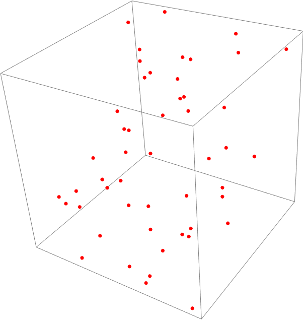
The notion of linearity imposes order on a system that otherwise appears random. Introducing a linear relationship between the fixed p₀, v₁ and v₂ vectors and the "random" 𝑎 and b through the parametric equation, results in points which fall on a common plane. Random is in quotes because the points are not completely random given that they are all forced onto a plane by the interaction with the vectors.
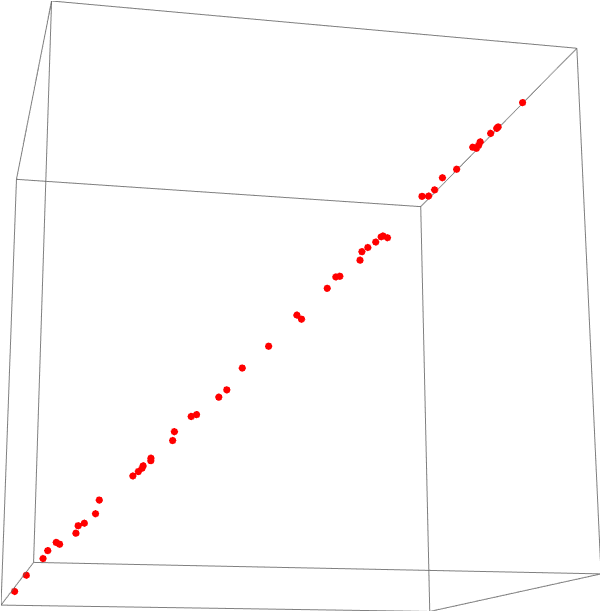
Below we rotate the graphic from above so that we see a "side view" of the cluster of points. It is clear that they are all on a single plane in the box which represents ℝ³ space.
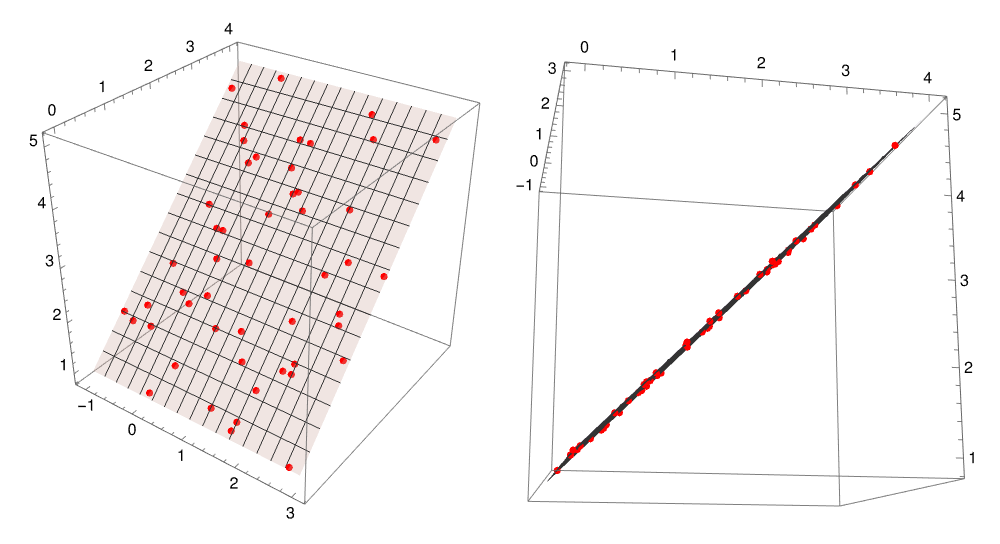
The illustrations above show only 50 points. Extending that to the plane described by the equation p = p₀ + 𝑎*v₁ + b*v₂ means choosing all possible points resulting from all possible values (between -2 and 2) that 𝑎 and b could take. Below on the left the same points in the graphic above are shown along with the parametric plot; on the right is the graphic on the left is again rotated to show the edge of the plane and the arrangement of all points on it.
Unknown variables x₁, x₂, … , xn are also called the independent variables because they could be chosen arbitrary with only one condition that the expression in the left-hand side of Eq.\eqref{EqRow.1} is equal to the given constant term b. Any characters can be used for their notation, either indexed (what we prefer) or unlabeled. So Eq.\eqref{EqRow.1} can be written as
Since coefficients 𝑎₁, 𝑎₂, … , 𝑎n can be any scalars including zeroes, an expression of the form
There are two particular cases that admit visualization of solutions to linear equation.
Flatten removes extra curly brackets in the output , but provides a warning message:
{y -> 4/3 - (2 x)/3}
{y -> 4/3 - (2 x)/3}
Reduce is often better than Solve
|
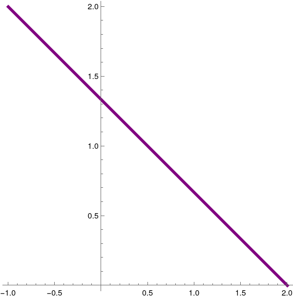
We plot the hyperplane (which is a line) in ℝ² using the following Mathematica script.
Labeled[ContourPlot[{2*x + 3*y == 4}, {x, -2, 2}, {y, -2, 2},
ContourStyle -> {Purple, Thickness[0.01]}, PlotRange -> All,
Axes -> True, Frame -> False], "Figure 4: Solution of 2D equation."]
|
In three-dimensional space, a linear equation \[ a\,x + b\, y + c\, z = d \] defines a hyperplane in ℝ³. For example, let us consider the equation \[ 2\, x - 3\, y + 4\, z = 5, \qquad x,y,z \in \mathbb{R} . \]
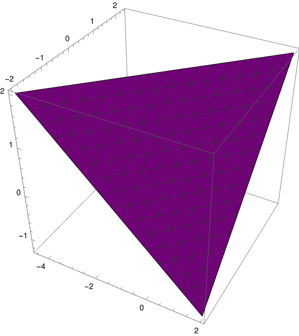
|
We plot the hyperplane (which is a plane) in ℝ³ using the following Mathematica script.
Labeled[ContourPlot3D[
2*x - 3*y + 4*z == 5, {x, -5, 2}, {y, -2, 2.5}, {z, -2, 2},
ContourStyle -> {Purple, Thickness[0.01]}, PlotRange -> All,
Axes -> True], "Figure 5: Solution of 3D equation."]
|
Now it is right time to discuss why solution set for 2D equation 𝑎 x + b y = c is a line (one-dimensional) while the plot of the linear equation 𝑎 x + b y + c z = d is a plane (two-dimensional). The reason lies in the fact that equation 𝑎 x + b y = c has one free variable and one dependent variable. The number of free variable of the linear equation in 3D is the number of degrees of freedom (which is the number of free variables (not containing pivots) in its row echelon form) in expressing the solution, so this number is two.
By independent variables we mean variables that do not depend on any constraint. By dependent variable, we mean variables that do depend on other variables or some constraints. If we see an expression such as z = f(x, y), then variable z is definitely a dependent variable because it depends on two other variables, x and y. Now it should be clear that a general linear equation
If, for instance, 𝑎n ≠ 0, the points in ℝn of the form
Each of m equations defines a hyperplane in n-dimensional space. Then the simultaneous solution or intersection set to a system of m linear equations is a geometric object of dimension at most n − m.
Since we discussed the two-dimensional case in the opening section, we just outline the main results. In xy-plane ℝ², a linear equation 𝑎 x + b y = c defines a straight line, which is a one-dimensional geometric object. The intersection set of two lines is usually a point---which is zero dimensional. If two lines are parallel and overlap, their intersection will be one-dimensional object---the line itself. However, if two lines are parallel, their intersection is empty (no dimension because cardinality of ∅ is zero).
A plane as a solution set of one linear equation 𝑎 x + b y + c z = d is two-dimensional. The intersection set of two planes is usually a one dimensional line unless they are parallel. Their intersection could be two-dimensional if two planes overlap or the empty set when they are parallel. The intersection set of three planes is usually a point that is zero dimensional. One can think of this situation as first intersecting two planes that results in a line and then intersecting the resulting line with the third plane, which is usually a point. The intersection set could also be the plane itself, which is two-dimensional, a line that is one-dimensional, or the empty set with no dimension. The intersection set of four planes is usually empty and has no dimension, although the intersection set could be of any dimension two or lower. Hopefully, you see a pattern developing in the following examples.
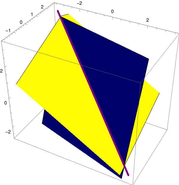
The equation of this line of intersection can be found with the aid of Mathematica. Since there is only one free variable, it is up to you which one you choose. Let us start with z as an independent variable

|
We plot the intersection of hyperplanes in ℝ³ using the following Mathematica script.
E1 = 3*x - 2*y + 5*z == 1;
E2 = 2*x + 7*y - 3*z == 2; twoPlanes = ContourPlot3D[Evaluate[{E1, E2}], {x, -3, 3}, {y, -3, 3}, {z, -3, 3}, ContourStyle -> {Yellow, Blue}, Mesh -> None, AspectRatio -> 1]; Labeled[%, "Figure 6: Intersection of two hyperplanes in Example 2."] |
|
solnline = Solve[{E1, E2}, {x, y}][[1]]
{x -> 1/25 (11 - 29 z), y -> 1/25 (4 + 19 z)}
solplot =
ParametricPlot3D[{x /. solnline[[1]], y /. solnline[[2]],
z}, {z, -2.5, 3.2}, PlotStyle -> {{Purple, Thickness[0.01]}}];
Show[solplot, twoPlanes] |
To solve the given system of linear equations by hand, we must first decide which variable we would like expressed in terms of the others. With our current system of two equations and three unknowns, we should be able to express two variables as a function of the third one in the final solution. We will choose to express the y and z variables in terms of x. A very simple way to do this is to move the x variable, along with its coefficient, to the right-hand side (RHS) of each equation. If we focus on the resulting left-hand side (LHS), then we obtain the problem with just two variables: \[ \begin{split} -2\,y + 5\,z &= 1 - 3\,x , \\ 7\,y - 3\, z &= 2- 2\,x . \end{split} \] To solve this system manually, we employ Chiò’s method; so we multiply the first equation by 7 and the second one by 2 and then add them. \[ \begin{split} 7 \left( -2\,y + 5\,z \right) &= 7 - 21\,x , \\ 2 \left( 7\,y - 3\, z \right) &= 4- 4\,x , \\ \hline 29\, z &= 11 - 25\, x . \end{split} \] Hence, from last equation, we obtain \[ z = \frac{1}{29} \left( 11 - 25\, x \right) . \] Substituting this expression into the first equation, we determine the value of another variable y.
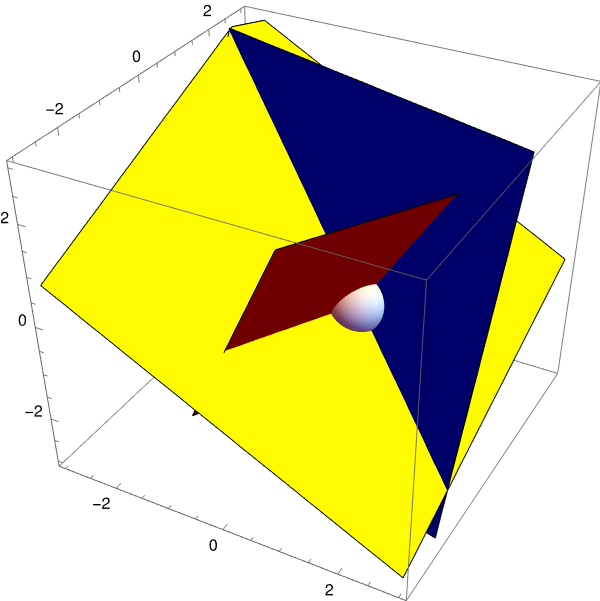
E2 = 2*x + 7*y - 3*z == 2;
E3 = 5*x - 3*y - 2*z == 4;
soln = Solve[{E1, E2, E3}, {x, y, z}][[1]]
solpointplot = Graphics3D[{White, Sphere[solpoint, 0.8]}];
Show[{twoPlanes, thirdPlane, solpointplot}, PlotRange -> {{-3, 3}, {-3, 3}, {-3, 3}}, AspectRatio -> 1]
Duality in matrix/vector multiplication
- If A and b are the matrix and vector given by \[ {\bf A} = \begin{bmatrix} -1& -2& 3 & 1 \\ 7 & 5 & 6 & 1 \\ 9 & -2 & 3 & 4 \end{bmatrix} \quad \mbox{and} \quad {\bf b} = \begin{bmatrix} -1 \\ 2 \\ 8 \\ 5 \end{bmatrix}. \] What linear system (written out in full) corresponds to the vector equation A x = b ?
- If A and b are the matrix and vector given by \[ {\bf A} = \begin{bmatrix} 1&2&-3&7 \\ 9 &8&2&-3 \\ 2&5& -7 & 3 \end{bmatrix} \quad \mbox{and} \quad {\bf b} = \begin{bmatrix} 5 \\ 4 \\ 3 \\ 1 \end{bmatrix}. \] What linear system (written out in full) corresponds to the vector equation A x = b ?
- Find the coefficient matrix A, the variable vector x, and the right-hand side vector b for the following systems. \[ {\bf (a)\ \ \ } \begin{split} 3\,x_1 -2\,x_2 + 5\,x_4 &= 21, \\ 2\,x_2 - 4\,x_3 + x_5 &= -7 , \\ - x_1 + 3\,x_3 - 6\,x_4 &= 13; \end{split} \qquad {\bf (b)\ \ \ } \begin{split} x_1 - 3\,x_2 + 2\,x_3 - x_4 &= 22, \\ 3\,x_1 + x_2 - 2\, x_3 + 4\,x_4 &= -8, \\ -x_1 - 4\,x_2 + 3\,x_3 - 5\, x_4 &= 78. \end{split} \]
- Let x = (x, y, z) . Express the “row problem” \[ \begin{split} {\bf a}^{\ast}_1 ({\bf x}) &= -1 , \\ {\bf a}^{\ast}_2 ({\bf x}) &= 4 , \\ {\bf a}^{\ast}_3 ({\bf x}) &= 1 , \end{split} \] as a linear system, assuming that a₁ = (2, −4, 5), a₂ = (3, 1, −2), and a₃ = (−4, 5, 2).
- Let x = (x, y, z) . Express the “row problem” \[ \begin{split} {\bf a}^{\ast}_1 ({\bf x}) &= -7 , \\ {\bf a}^{\ast}_2 ({\bf x}) &= 14 , \\ {\bf a}^{\ast}_3 ({\bf x}) &= 31 , \end{split} \] as a linear system, assuming that a₁ = (2, −3, 2), a₂ = (3, 1, −9), and a₃ = (−1, 3, 6).
- Express the linear system below in “row” form \[ \begin{split} 2\,x - 3\,y + 5\,z &= 2, \\ 3\,x - 6\,y + 9\, z &= 8, \\ -x + 2\,y - 7\,z &= 3. \end{split} \]
- Express the linear system below in “column” form \[ \begin{split} -x + 9\,y + 2\, z &= 21 , \\ 2\,x - 8\,y + 3\,z &= 15, \\ 3\,x + 4\,y - 8\,z &= 27. \end{split} \]
- Express the “column problem” \[ {\bf a}_1 x_1 + {\bf a}_2 x_2 + {\bf a}_3 x_3 = {\bf b} \] as a linear system in the variables x₁, x₂, x₃, assuming a₁ = [6, −3, 5]T, a₂ = (7, 2, −3]T, and a₃ = [−2, 4, 3]T.
- Express the “column problem” \[ u\,{\bf a}_1 + v\,{\bf a}_2 + w\, {\bf a}_3 = {\bf b} \] as a row problem, where a₁ = [3, −1, 4]T, a₂ = (3, 8, −9]T, a₃ = [−4, 5, 6]T, and b [3, 2, 5]T.
- What linear combinations (if any) of the vectors (3, 1, 2, 4), (1, 6, 5, 3), and (4, 3, 1, 6) add up to (7, −2, 5, 3)?
-
Find the matrix that results from performing the indicated elementary row
operation.
- \( \displaystyle \begin{bmatrix} 2&7&4 \\ 0&3&1 \\ 3&2&3 \end{bmatrix} \qquad \) R3 ← R3 + (−3/2)·R1;
- \( \displaystyle \begin{bmatrix} 1&7&3 \\ 2&3&-1 \\ 0&4&6 \end{bmatrix} \qquad \) R2 ← R2 −2·R1;
- \( \displaystyle \begin{bmatrix} 3&4&2 \\ 0&1&7 \\ 1&3&8 \end{bmatrix} \qquad \) R3 ← R3 + (−1/3)·R1;
- \( \displaystyle \begin{bmatrix} 1&2&6 \\ 0&1&5 \\ 0&4&3 \end{bmatrix} \qquad \) R3 ← R3 −4·R2;
- \( \displaystyle \begin{bmatrix} 7&6&5 \\ 0&4&3 \\ 0&2&7 \end{bmatrix} \qquad \) R3 ← R3 −2·R2;
- \( \displaystyle \begin{bmatrix} 1&5&2 \\ 0&1&1 \\ 0&7&4 \end{bmatrix} \qquad \) R3 ← R3 −7·R2.
-
Find the matrix that results from performing the indicated elementary row
operation.
- \( \displaystyle \begin{bmatrix} 3&0&8 \\ 2&-4&2 \end{bmatrix} \qquad \) R1 ↑ R2;
- \( \displaystyle \begin{bmatrix} 1&2&3&4 \\ 0&3&5&2 \\ 3&7&0&4 \end{bmatrix} \qquad \) R3 ← R3 − 3·R1;
- \( \displaystyle \begin{bmatrix} 1&3&4&2&1 \\ 0&1&5&2&3 \\ 0&-1&4&2&-1 \end{bmatrix} \qquad \) R3 ← R3 − ;R1;
- \( \displaystyle \begin{bmatrix} 1&2&-4&5 \\ 0&3&8&10 \end{bmatrix} \qquad \) R2 ← R2 + 2·R1;
- \( \displaystyle \begin{bmatrix} 1&1&3 \\ 5&5&21 \end{bmatrix} \qquad \) R2 ← R2 − 5·R1;
- \( \displaystyle \begin{bmatrix} 1&-2&5&7 \\ 0&1&3&5 \\ 0&0&1&3 \end{bmatrix} \qquad \) R3 ← R3 + (−1/2)·R2.
-
identify the elementary row operation (by Type and by action) that transforms the
matrix on the left into the matrix on the right.
- \( \displaystyle \begin{bmatrix} 3&1&2&3 \\ 1&2&1&5 \end{bmatrix} \qquad \) and \( \displaystyle \quad \begin{bmatrix} 3&1&2&3 \\ 1&2&1&5 \end{bmatrix} \qquad \)
- \( \displaystyle \begin{bmatrix} 1&2&3&1 \\ 0&2&1&2 \\ 0&6&3&7 \end{bmatrix} \qquad \) and \( \displaystyle \quad \begin{bmatrix} 1&2&3&1 \\ 0&2&1&2 \\ 0&0&0&1 \end{bmatrix} \qquad \)
- \( \displaystyle \begin{bmatrix} 1&2&2&2&4 \\ 3&2&1&3&3 \\ 0&1&1&2&2 \\ 0&4&2&2&1 \end{bmatrix} \qquad \) and \( \displaystyle \quad \begin{bmatrix} 1&2&2&2&4 \\ 3&2&1&3&3 \\ 3&0&-1&-1&-1 \\ 0&1&1&2&2 \\ 0&4&2&2&1 \end{bmatrix} \qquad \)
- \( \displaystyle \begin{bmatrix} 1&2&1&5 \\ 0&-5&-1&-12 \end{bmatrix} \qquad \) and \( \displaystyle \quad \begin{bmatrix} 1&2&1&5 \\ 0&1&0.2&2.4 \end{bmatrix} \qquad \)
- \( \displaystyle \begin{bmatrix} 1&2&1&5 \\ 3&1&2&3 \end{bmatrix} \qquad \) and \( \displaystyle \quad \begin{bmatrix} 1&2&1&5 \\ 0&-5&-1&-12 \end{bmatrix} \qquad \)
- \( \displaystyle \begin{bmatrix} 1&2&1&5 \\ 0&1&0.2&2.4 \end{bmatrix} \qquad \) and \( \displaystyle \quad \begin{bmatrix} 1&0&0.6&0.2 \\ 0&1&0.2&2.4 \end{bmatrix} \qquad \)
- Determine whether or not the given vector is a solution to the system: \[ \begin{split} x+ 2\,y - 3\, z &= 0 , \\ 2\,x - 3\,y + z &= 0 . \end{split} \] \[ {\bf (a)\ \ } \left( 3, 3, 3 \right) , \qquad {\bf (b)\ \ } \left( 1, 2, 3 \right) . \]
- Determine whether or not the given vector is a solution to the system: \[ \begin{split} x + 2\, y - 4\,z &= 0, \\ 3\,x = 5\,y + 2\, z &= 0 . \end{split} \] \[ ({\bf a}) \quad \begin{bmatrix} 11 \\ 16 \\ 14 \end{bmatrix} , \qquad ({\bf b}) \quad \begin{bmatrix} 16 \\ 14 \\ 11 \end{bmatrix} , \qquad ({\bf c}) \quad \begin{bmatrix} 14 \\ 16 \\ 11 \end{bmatrix} . \]
- Determine whether or not the given vector is a solution to the system: \[ \begin{split} x + 2\, y - 4\,z &= 3, \\ 3\,x = 5\,y + 2\, z &= 2 . \end{split} \] \[ ({\bf a}) \quad \begin{bmatrix} 9 \\ 7 \\ 5 \end{bmatrix} , \qquad ({\bf b}) \quad \begin{bmatrix} 16 \\ 14 \\ 11 \end{bmatrix} , \qquad ({\bf c}) \quad \begin{bmatrix} 4 \\ 6 \\ 11 \end{bmatrix} . \]
- Show that the following pairs of matrices are row equivalent by finding a sequence of one or more elementary row operations that transforms the first matrix into the second matrix. \[ ({\bf a})\quad \begin{bmatrix} 1&3&2 \\ 0&1&1 \end{bmatrix} , \quad \begin{bmatrix} 1&0&-1 \\ 0&1&1 \end{bmatrix} ; \qquad ({\bf b})\quad \begin{bmatrix} 2&7&1 \\ 1&5&4 \end{bmatrix} , \quad \begin{bmatrix} 1&5&4 \\ 2&7&1 \end{bmatrix} ; \] \[ ({\bf c})\quad \begin{bmatrix} 1&1&3 \\ 0&1&1 \\ 0&0&1 \end{bmatrix} , \quad \begin{bmatrix} 1&0&0 \\ 0&1&0 \\ 0&0&1 \end{bmatrix} ; \qquad ({\bf d})\quad \begin{bmatrix} 1&2&1 \\ 2&0&3 \\ 3&7&4 \end{bmatrix} , \quad \begin{bmatrix} 1&2&1 \\ 0&-4&1 \\ 0&1&1 \end{bmatrix} ; \] \[ ({\bf e})\quad \begin{bmatrix} 1&3&1&5 \\ 1&0&-11&-1 \\ 0&4&2&1 \\ 0&0&1&2 \end{bmatrix} , \quad \begin{bmatrix} \end{bmatrix} ; \qquad ({\bf f})\quad \begin{bmatrix} \end{bmatrix} 1&0&1 \\ 0&1&2, \quad \begin{bmatrix} 1&2&5 \\ 2&5&12 \end{bmatrix} . \]
- Anton, Howard (2005), Elementary Linear Algebra (Applications Version) (9th ed.), Wiley International
- Beezer, R., A First Course in Linear Algebra, 2015.
- Beezer, R., A Second Course in Linear Algebra, 2013.
- Boelkins, M.R., Goldberg, J.I., Potter, M.C., Differential Equations with Linear Algebra, Mathematica Help, 2009.
- Osgood, William F. (1919). "The life and services of Maxime Bôcher". Bull. Amer. Math. Soc. 25 (8): 337–350. doi:10.1090/s0002-9904-1919-03198-x.