Although the topic of this section is related to affine geometry, it helps the reader to appreciate the geometrical ideas underlying and motivating linear algebra. We do not discuss practical applications of drawing lines in multidimensional spaces, instead we refer to famous Bresenham's and Wu's algorithms for accomplishing this task.
Lines and Planes
Lines in ℝ²
Lines in ℝ² can be explicitly described in either parametric or Cartesian form.
Theorem 1:
The following sets are lines in ℝ².
Lp = { p + tw : t∈ℝ} with p, w ∈ ℝ² and w≠0
(parametric form)
Lc = { x ∈ ℝ² : n • x = b } with n ∈ ℝ², b ∈ ℝ, n ≠ 0
(Cartesian form).
Here n = (n₁, n₂) is a normal vector for the line, and dot "•" stands for the dot product, n • x = n₁x₁ + n₂x₂.
Instead of dot product, this form can also be written as y = m x + b for some real m, b ∈ ℝ.
Every line can be written in the form (i) or (ii). If n ⊥ w (so n • w = 0) and b = n • p, then Lp = Lc.
First, we show the equality, Lp = Lc, under the stated conditions. Lp ⊂ Lc : Start with an element x =
p + tw ∈ Lp. Multiply this equation with n (keeping in mind that n • w = 0) leads to n • x = n • p = b, which shows that x ∈ Lc.
Lc ⊂ Lp : Conversely, consider an element x ∈ Lc, which by definition, satisfies n • x = b. Given that b = n • p, this equation can be re-written as n • (x − p) = 0. Every vector x − p can be represented as a linear combination x − p = cn + tw (since (n, w), as
two non-zero orthogonal vectors, form a basis of ℝ²). From 0 = n • (x − p) = c |n|², we
conclude that cx = p + tw ∈ Lp.
It is clear that every line p + W can be written in parametric form by choosing a non-zero vector w ∈ ℝ² such that W = span(w). Conversely, every parametric form
defines a line by setting W = span(w).
To complete the proof, we show that every line in parametric form can be converted into Cartesian form and vice versa. To see the former, start with vectors p, w defining a parametric line Lp. Setting n so that n ⊥ w, and b = n • p defines a line in Cartesian form with Lc = Lp. If we start with the Cartesian line Lc, specified by n and b, then setting w = n⊥ and choosing p to be any solution of n • p = b, we get a parametric line Lp with Lp = Lc.
The geometric interpretation of the various vectors which enter the parametric and Cartesian form is indicated in the following figure.
Line in ℝ² with parametric form
Figure 11.1, Oxford, page 120
code:
For the parametric form, x(t) = p + tw, the vector p is a vector ’to the line’ and the vector w a vector ’along the line’. For the Cartesian form n • x = b, the vector n is a vector orthogonal to the line while |b|/|n| is the minimal distance of the line from the origin. To verify the last statement, write the parametric form of a line as
\[
|{\bf n}| \, |{\bf x}| \,\cos\left( \angle ({\bf n}, {\bf x}) \right) = b .
\]
The value of |x| is minimal when |cos(∢(n, x))| takes its maximal value which is, of
course, |cos(∢(n, x)) = 1. It follows that the minimal value of |x| is indeed |b|/|n|.
We should stress that neither the parametric nor the Cartesian form of a line is unique, that is, one and the same line can be described by different equations of this form.
For example, in the parametric form we can use instead of w any non-zero multiple
βw or, instead of p any other vector p + αw to the line. For the Cartesian form,
using αn and αb instead of n and b describes the same line. Theorem 1 indicates
a method to convert a line in parametric form to Cartesian form and vice versa. It is
worth practicing this by looking at examples.
Example 1:
Let us consider the line 2y = x. Any point (x, y) on this line must satisfy equation, and all points that satisfy the equation are on this line.
Line in ℝ²
Figure
code:
Another way to describe the points on the line is by giving their position vectors. We can let x = t, where t is any real number. Then y is determined by y = x/2 = t/2. So x = (x, y) is the position vector of a point on the line, then
\[
{\bf x} = \begin{pmatrix} 2t \\ t \end{pmatrix} = t \begin{pmatrix} 2 \\ 1 \end{pmatrix} = t{\bf w} , \qquad t \in \mathbb{R} .
\]
For example, if t = 2.5, we get the position vector of the point (5, 2.5) on the line, and if t = −2, we obtain the point (−4, −2). As the parameter t runs through all real numbers, this vector equation gives the position vectors of all the points on the line.
Starting with the parametric vector equation
\[
{\bf x} = \begin{pmatrix} x \\ y \end{pmatrix} = t{\bf w} = t \begin{pmatrix} 2 \\ 1 \end{pmatrix} , \qquad t \in \mathbb{R} ,
\]
we can retrieve the Cartesian equation using the fact that the two vectors are equal if and only if their components are equal. This gives us the two equations x = 2t and y = t. Eliminating the parameter t between these two equations yields 2y = x.
End of Example 1
Example 2:
Consider the line 2y = x + 3. Proceeding as above, we set
x = t, t ∈ &reals. Then 2y = x + 3 = t + 3, so the position vector of a point on the line is given by the parametric form
We convert this line into Cartesian form by setting p = (0, 3/2), w = (2, 1), and x = (x, y). We choose n so that n • w = 0; for instance, let n = (−1, 2), then n ⊥ w. Hence, b = n • p = 3, and the Cartesian form of the line becomes
Its minimal distance from the origin is |b|/|n| = 3/√5.
End of Example 2
Example 3:
A line in Cartesian form is given by 3x −5y = 4. We can write this equation as n • x = b with n = (3, −5), x = (x, y), and b = 4. A vector w along the line is found by w = n⊥ = (5, 3). To find a vector p to the line we can
use any solution to the Cartesian equation; for example, p = (3, 1). Hence, a parametric form of the line becomes
We can interpret this equation as follows. To locate any point on the line, first locate one particular point p that is on the line.; for instance, the y intercept (0, −4/5). Then the position vector of any point x on the line is a sum of two displacements, first going to the point on the line p and then going along the line, in a direction parallel to the vector w.
End of Example 3
Example 4:
Convert the parametric form
\[
{\bf x}(t) = \begin{pmatrix} 2 \\ 1 \end{pmatrix} + t \begin{pmatrix} \phantom{-}3 \\ -1 \end{pmatrix}
\tag{4.1}
\]
of a line into Cartesian form. Find the minimal distance of the line from the origin.
Solution: With p = (2, 1), w = (3, −1), and x = (x, y), we have n = w⊥ = (1, 3) and b = n • p = 5. Hence, the Cartesian form of the line is
\[
\begin{pmatrix} 1 \\ 3 \end{pmatrix} \bullet {\bf x} = 5 \qquad \mbox{or}\qquad x + 3y = 5.
\]
Its minimal distance from the origin is \( \displaystyle |b|/\sqrt{|{\bf n}|} = 5\sqrt{3^2 + 1^2} = \sqrt{5/2} \approx 1.58114 . \)
End of Example 4
The intersection of two lines in ℝ² can be discussed using either parametric or Cartesian forms. We opt for the latter and write the equations for the two lines as
Evidently, the intersection L1 ∩ L2 is determined by the solution to two simultaneous
linear equations in two variables. With n1 = (n11, n12), n2 = (n21, n22), and x = (x, y), these equations can also be written as
\[
n_{11} x + n_{12} y = b_1 , \qquad n_{21} x + n_{22} y = b_2 ,
\]
or, in matrix-vector form, as Nx = b, where N is a 2 × 2 matrix with entries nij and b = (b1, b2).
We already know from the introduction that there are three possibilities for the solutions to a system of two linear equations in two variables. The solution can be unique, but we can also have an entire line of solutions or there may be no solution at all, depending on the coefficients in the linear equations. In geometrical terms, these three cases correspond to the two lines intersecting in a point, being identical and being parallel.
Lines in ℝ³
It is natural to identify points on a line in ℝ³ in parametric form. Again, we need a point p to pass through and the direction or in the opposite direction. w of the line. Therefore, a line in ℝ³ is given by a vector equation with one parameter,
where x is the position vector of any point on the line, p is the position vector of one particular point on the line, and w is the direction of the line, Using Cartesian coordinate, we write line's equation as
\begin{equation} \label{EqLine.1}
{\bf x} = \begin{pmatrix} x \\ y \\ z \end{pmatrix} = \begin{pmatrix} p_1 \\ p_2 \\ p_3 \end{pmatrix} + t \begin{pmatrix} w_1 \\ w_2 \\ w_3 \end{pmatrix} , \qquad t\in \mathbb{R} .
\end{equation}
Theorem 2:
The following sets are lines in ℝ³.
Lp = { p + tw : t ∈ ℝ } with p, w ∈ ℝ³ and w ≠ 0.
Lc = { x ∈ ℝ³ : n₁ • x = b₁, n₂ • x = b₂ }
with n₁, n₂ linearly independent, b₁, b₂ ∈ ℝ.
All lines in ℝ³ can be written in the form (i) and (ii). If {w, n₁, n₂} is a basis of
mutually orthogonal vectors and b₁ = n₁ • p, b₂ = n₂ • p, then Lp = Lc.
We begin by showing the equality of the two sets.
Lp ⊂ Lc : Start with x = p + tw ∈ Lp. Multiplying this equation with n₁ and n₂ gives
n₁ • x = n₁ • p = b₁ and n₂ • x = n₂ • p = b₂. Therefore, x ∈ Lc.
Lc ⊂ Lp : A vector x ∈ Lc satisfies ni • x = bi, or, equivalently, ni • (x − p) = 0 for i = 1, 2. We can write the vector x − p as a linear combination of the basis {w, n>₁, n>₂}, so x − p = tw + α₁n>₁ + α₂n>₂. It follows that
and hence αi = 0 for i = 1, 2. Therefore, x = p + tw ∈ Lp.
Clearly, every line p + W can be written in parametric form by choosing a vector w, then W = Span(w); conversely, every parametric form given a line with W = Span(w).
Given a parametric line Lp, specified by vectors p, w, we can find mutually orthogonal vectors w, n₁, n₂. Then n₁, n₂ along with b₁ = n>₁ • p and b₂ = n₂ • p define a Cartesian line Lc with Lc = Lp.
Conversely, let Lc be a Cartesian line specified by
n₁, n₂ and b₁, b₂. Define w = n₁ × n₂. We can always find a solution p to the equations n₁ • p = b₁ and n₂ • p = b₂. Then w and p define a parametric line Lp with Lp = Lc.
We can also describe a line in ℝ³ by Cartesian equations, but this time we need two such equations because there are three variables. Equating components in the vector equation \eqref{EqLine.1}, we have
The two Cartesian equations for a line, n₁ • x = b₁ and n₂ • x = b₂,
can also be written as a linear system N x = b with two equations and three variables, where N is the matrix with entries nij and b = (b₁, b₂). From this point of view, the
line is the solution space of the linear system. This is another illustration of the close
relation between affine k-planes and linear systems.
Theorem 3:
Let L = {p + tw : t ∈ ℝ} ⊂ ℝ³ be a line in parametric form and
p₀ ∈ ℝ³. The minimal distance of p₀ from the line arises at tmin = −d • w/|w|², where
d = p − p₀. The minimal distance is given by dmin = |d × w|/|w|.
We simply work out the distance square d²(t) = |x − p₀|² of an arbitrary
point x(t) = p + tw on the line from the point p₀. This leads to
This is minimal when the expression inside the square bracket vanishes which happens for t = tmin = −d • w/|w|²'. This proves the first part of the claim. For the second part we simply compute the distance at tmin,
which gives
This is a line parallel to the xy-plane in ℝ³. The direction vector has a zero in the third component, so there is no change in the z direction: the z coordinate has the constant value z = 1.
End of Example 6
In ℝ², two lines are either parallel or intersect in unique point. In ℝ³, more can happen. Two lines in ℝ³ either intersect in a unique point, are parallel or are skew, which means that they do not intersect and are not parallel.
One way to imagine skew lines is to look around: do you see ceiling and floor? Now draw one line on the ceiling and another one on the floor. Most likely they will be skewed because it is difficult to plot them parallel. You can also draw two skew lines on two walls or a wall and a floor.
Two lines are said to be coplanar if they lie in the same plane, in which case they are either parallel or intersecting.
A parametric form of a given line is not unique: we can in
fact change the point p = (p₁, p₂, p₃) used in the representation \eqref{EqLine.1}, choosing it
arbitrarily among all the infinite points of the line, or we can multiply the parameter t for an arbitrary nonzero constant: in both the cases the line does not change, even
though its parametric equations can take a different form.
Example 7:
Let us consider two lines written in parametric form:
\[
L_1 \ : \quad \left[ \begin{array}{c} x \\ y \\ z \end{array} \right] = \begin{pmatrix} 1 \\ 2 \\ 3 \end{pmatrix} + t \begin{pmatrix} \phantom{-}4 \\ \phantom{-}2 \\ -2 \end{pmatrix} , \qquad t \in \mathbb{R} ,
\]
and
\[
L_2 \ : \quad \left[ \begin{array}{c} x \\ y \\ z \end{array} \right] = \begin{pmatrix} 3 \\ 4 \\ 5 \end{pmatrix} + t \begin{pmatrix} -2 \\ -1 \\ \phantom{-}1 \end{pmatrix} , \qquad t \in \mathbb{R} .
\]
These two lines L₁ and L₂ have the same direction, since the direction vector of the first line (4, 2, −2) is a multiple of another one, (−2, −1, 1). Therefore, the two lines are parallel or they coincide. To establish their mutual positions,
it is sufficient to check if the starting point p = (1, 2, 3) of the first line belongs to the line L₂, so we need to check whether there exists t such that
Therefore, we conclude that the given lines L₁ and L₂ are parallel.
Let us convert parametric equations of lines L₁ and L₂ into Cartesian form. Excluding t form equations of L₁, we get
\[
t = \frac{x-1}{4} = \frac{y-2}{2} = \frac{z-3}{-2}
\]
This yields
\[
\begin{cases}
x &= 2y -3 , \\
y &= -z +5 .
\end{cases}
\]
Similarly for L₂, we have
\[
t = \frac{x-3}{-2} = \frac{y-4}{-1} = \frac{z-5}{1} \qquad \Longrightarrow \qquad \begin{cases}
x &= 2y - 5 , \\
y &= -z +9 .
\end{cases}
\]
End of Example 7
Example 8:
Let us consider two lines written in parametric form:
\[
L_1 \ : \quad \left[ \begin{array}{c} x \\ y \\ z \end{array} \right] = \begin{pmatrix} \phantom{-}1 \\ \phantom{-}0 \\ -1 \end{pmatrix} + t \begin{pmatrix} \phantom{-}2 \\ \phantom{-}1 \\ -1 \end{pmatrix} , \qquad t \in \mathbb{R} ,
\]
and
\[
L_2 \ : \quad \left[ \begin{array}{c} x \\ y \\ z \end{array} \right] = \begin{pmatrix} \phantom{-}3 \\ -1 \\ \phantom{-}2 \end{pmatrix} + t \begin{pmatrix} \phantom{-}1 \\ \phantom{-}2 \\ -1 \end{pmatrix} , \qquad t \in \mathbb{R} .
\]
First, we check whether these two lines intersect at a point. To answer this question, we substitute the position vector p = (1, 0 , −1) into the equation of the second line. This leads to the system of linear equations
On a line, there is essentially one direction in which a point can move, given as all possible scalar multiples of a given direction, but on a plane there are more possibilities. A point can move in two different directions, and in any linear combination of these two directions.
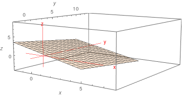
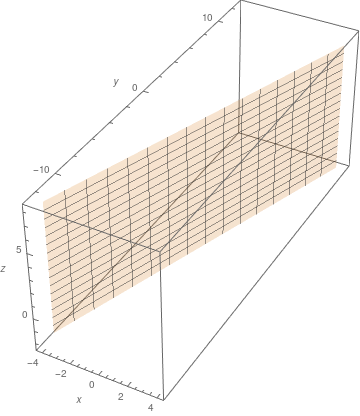
Planes are sets of the form P = p + W ⊂ ℝ³, where p ∈ ℝ³ and W ⊂ ℝ³ is a
two-dimensional vector subspace.
Clear[a, b, c, d, x0, y0, z0, v, w, k, q, r, s]
a := 3;
b := -1;
c := 0;
x0 := 1;
y0 := 3;
z0 := 2;
d := {a, b, c}.{x0, y0, z0};
planePlot2 =
ParametricPlot3D[{u, (d - a u)/b, v}, {u, -4, 4}, {v, -2, 8},
PlotStyle -> Opacity[0.2], AxesLabel -> {x, y, z}]
Plane ≌ ℝ3
Theorem 4:
The following sets are planes in ℝ³.
Pp = { p + tw₁ + sw₂ : t, s ∈ ℝ }
with p ∈ ℝ³ and w₁, w₂ ∈ ℝ³ are linearly independent;
Pc = { x ∈ ℝ³ : n • x = b }
with n ∈ ℝ³ nonzero, b ∈ ℝ.
Every plane can be written as in (i) or (ii). If n ⊥ w₁, w₂ and b = p • n, then Pp = Pc.
As in theorem 1, we begin by showing that Pp = Pc under the stated conditions. Pp ⊂ Pc : For a vector x = p + tw₁ + sw₂, take the dot product with n, keeping in mind that n • w₁ = n • w₂ = 0. This leads to n • x = n • p = b, so that x ∈ Pc.
Pc ⊂ Pp : Start with a vector x ∈ Pc, so that n • x = b, or, equivalently, n • (x −p) = 0. To solve this last equation we first note that {n, w₁, w₂} forms a basis of ℝ³. This means that we can write every vector x −p as a linear combination x −p = cn + tw₁ + sw₂. From 0 = n • (x −p) = c|n|², it follows that c = 0 and, hence, x = p + tw₁ + sw₂ ∈ Pp.
Every plane p + W can be written in parametric form by choosing a basis {w₁, w₂} of W. Conversely, a parametric form with w₁, w₂ defines a plane by setting W = span(w₁, w₂).
Every plane in parametric form can be converted into Cartesian form. Start with
vectors p, w₁, w₂, specifying a parametric plane Pp. Setting n = w₁ × w₂ and b = p • n defines a Cartesian plane Pc with Pc = Pp.
On the other hand, for a Cartesian plane Pc, specified by n and p, we can find mutually orthogonal vectors {n, w₁, w₂} together with any solution of p of n • p = b defines a parametric plane Pp with Pp = Pc.
In the parametric form, p is a vector ’to the plane’ while
w₁ and w₂ are vectors
’along the plane’. For the Cartesian form, n is a vector orthogonal to every vector in
the plane and |b|/|n| is the minimal distance of the plane from the origin.
The minimal distance from the origin is |b|/|n| = 1/√6 ≈ 0.408248.
N[1/Sqrt[6], 12]
0.408248290464
End of Example 9
Example 10:
Let us consider the plane x − 3y + 2z = 4. We identify a normal vector to the plane as n = (1, −3, 2) and b = 4. Upon setting x = (x, y, z), the plane equation can be written in the Cartesian standard form n • x = b. As a vector p ’to the plane’ we can use any vector that satisfies n • p = b = 4; for example, p = (2, 0, 1). To get two vectors w₁, w₂ ’in the plane,’ we need two linearly independent solutions to n • x = 0; for example, w₁ = (1, 1, 1) and w₂ = (3, 2, 1). Hence, a parametric form of the plane becomes
Theorem 5:
Suppose that an equation of a plane is given in either in Cartesian form by n • x = b or in parametric form by x(t, s) = p + tw₁ + sw₂. The minimal distance of the plane from p₀ ∈ ℝ³ is given by
\begin{equation} \label{EqLine.2}
d_{\min} = \frac{\left\vert b - {\bf n} \bullet {\bf p}_0 \right\vert}{|{\bf n}|} = \frac{|{\bf d} \bullet \left( {\bf w}_1 \times {\bf w}_2 \right) |}{|{\bf w}_1 \times {\bf w}_2 |} , \quad {\bf d} = {\bf p} - {\bf p}_0 .
\end{equation}
We start with the Cartesian form n • x = b and subtract n • p₀, so that n • (p − p₀) = b − n • p₀ or, equivalently,
\[
|{\bf n}| \, \left\vert {\bf x} - {\bf p}_0 \right\vert \cos ∢\left( {\bf n}, {\bf x} - {\bf p}_0 \right) = b - {\bf n} \bullet {\bf p}_0 .
\]
The value of |n − p0| is maximal when the (absolute) value of the cosine is 1, so that dmin = |b − n • p₀|/|n|. This proves the first part of Eq.\eqref{EqLine.2}. For the second part, simple insert the relations n = w₁ × w₂ and b = p • n.
Example 11:
Find the minimal distance of the plane 3x − 2y + z = 5 from p₀ = (−1, 1, 2).
Solution:
The plane is given in Cartesian form n • x = b, with n = (3, −2, 1) and b = 5. Inserting n • p₀ = −3, |n| = √14, and b = 5 into formula \eqref{EqLine.2}, we get
If the two vectors n 1 and n 2 are linearly independent then L is a line, written down in Cartesian form, as comparison with Theorem 2 shows. If n₁ and n₂ are linearly dependent, n₂ = αn₁ for a non-zero α ∈ ℝ, then the equations for the two planes turn into n₁ • x = b₁ and n₁ • x = b₂/α. If αb₁ = b₂, the two planes are identical and their intersection is the entire plane, so L = P₁ = P₂. On the other hand, if αb₁ ≠ b₂, then the planes are parallel and the intersection is empty, L = ∅.
Example 12:
Find the intersection of the two planes −x +2y − z = 3 and 3x − 𝑎y + 3z = b for all values of
the parameters 𝑎, b ∈ ℝ. If the intersection is a line, find its parametric form.
Solution:
We have n₁ = (−1, 2, −1),
b₁ = 3 and n₂ = (3, −𝑎, 3), b₂ = b.
(1) 𝑎 ≠ 6. In this case n₁ and n₂ are linearly independent and the intersection must be a
line. Withw = n₁ × n₂ = (6 −𝑎, 0, 𝑎 −6)
Cross[{-1, 2, -1}, {3, -aa, 3}]
{6 - aa, 0, -6 + aa}
and a special solution p = (0, 9+ b, 3𝑎 + 2b)/(6−𝑎)
Solve[{-x + 2*y - z == 3, 3*x - aa*y + 3*z == b}, {x, y, z}]
{{y -> -((9 + b)/(-6 + aa)), z -> -((3 aa + 2 b)/(-6 + aa)) - x}}
to the two equations the parametric form of the intersection line is
\[
{\bf x}(t) = \frac{1}{6-a} \begin{pmatrix} 0 \\ 9+b \\ 3a + 2b \end{pmatrix} + t \begin{pmatrix} \phantom{-}1 \\ \phantom{-}0 \\ -1 \end{pmatrix} , \qquad t \in \mathbb{R} .
\]
(2a) 𝑎 = 6 and b ≠ −9. In this case the two planes are parallel so the intersection is empty.
(2b) 𝑎 = 6 and b = −9. The two planes are identical.
End of Example 12
The intersection of a line and a plane in ℝ³ is easiest discussed with the line in parametric and the plane in Cartesian form, that is
\[
L = \left\{ {\bf p} + t{\bf w} \mid t \in \mathbb{R} \right\} , \qquad P = \left\{ {\bf x} \in \mathbb{R}^3 \mid {\bf n} \bullet {\bf x} = b \right\} .
\]
By inserting the parametrization of the line into the equation for the plane we find for the intersection
\[
L \cap P = \left\{ {\bf p} + t{\bf w} \mid \left( {\bf n} \bullet {\bf w} \right) t = b - {\bf n} \bullet {\bf p} \right\} .
\]
If n • w ≠ 0, then we can solve for t = t₀ = (b − n • p)/(n • w) and the intersection consists of a single point, L ∩ P = {p + t₀w}. On the other hand, ifn • w = 0 and b ≠ n • p, there is no solution for t, so the intersection is empty, L ∩ P = { }. For n • w = 0 and b = n • p. every t ∈ ℝ is a solution so that L ∩ P = L — the line is a subset of the plane.
Example 13:
Find the intersection of the plane with Cartesian equation 2x − 3y + 5z = 7 with the line in parametric form given by
\[
{\bf x} (t) = \begin{pmatrix} \phantom{-}2 \\ -3 \\ \phantom{-}1 \end{pmatrix} + t \begin{pmatrix} -3 \\\phantom{-}2 \\ -1 \end{pmatrix} , \qquad t \in \mathbb{R} .
\]
With x = (x, y, z), we can split the parametric form of the line into its components x = 2 −3t, y = −3 + 2t, z = 1 −t, and insert these into the equation for the plane. This gives
\[
2 \left( 2 -3t \right) -3 \left( -3 + 2t \right) + 5 \left( 1-t \right) = 7
\]
Hence, the intersection point is x(11/17) = (1, −29, −28)/17.
End of Example 13
Suppose that we are interested in the intersection P₁ ∩ P₂ ∩ P₃ of the three planes in ℝ³
in Cartesian form:
This intersection is clearly the same as the solution to the system of the three linear equations in three variables given by ni • x = bi for i = 1, 2, 3. Another example of
the close relationship between the geometry of affine k-planes and linear systems. Of course, the intersection can be found by solving the linear system explicitly. However, the qualitatively different cases which can arise can be easily reasoned out from what we have discussed so far.
Start by considering the intersection P₁ ∩ P₂ of the first two planes. This intersection may be a line, a plane or it may be empty. If L = P₁ ∩ P₂ is a line, then the triple intersection P₁ ∩ P₂ ∩ P₃ = L ∩ P₃ can be a point, a line or be empty. This already covers all the cases but one, which is the case P₁ = P₂ = P₃, so that the intersection
is a plane.
Example 14:
Let us find the intersection of the three planes with Cartesian equations 2x − y + 4z = 7, 4x − y + z = 1,
and 4x + 3y − 5z = 4.
Solve[{2*x - y + 4*z == 7, 4*x - 1*y + z == 1,
4*x + 3*y - 5*z == 4}, {x, y, z}]
{{x -> 3/4, y -> 9/2, z -> 5/2}}
From the first equation, we get y = 2x + 4z −7. Substituting y into two other equation, we obtain the system of two equations:
End of Example 14
Example 15:
Artificial neural networks are motivated by the structure of the human brain and they
play an important role in modern computing. Many of the operating principles of artificial
neural networks can be formulated and understood in terms of linear algebra. Here, we would like to introduce one of the basic building blocks of artificial neural networks — the
perceptron.
A Perceptron is a neural network unit that does certain computations to detect features or business intelligence in the input data. It is a function that maps its input “x,” which is multiplied by the learned weight coefficient, and generates an output value ”f(x)."
The structure of the perceptron is schematically illustrated in the figure below.
The perceptron receives an input vector x = (x1, x2, … , xn) ∈ ℝn, which it converts into a
real output y ∈ ℝ in two steps. In the first step, it transforms x as
where w ∈ ℝn is called the weight vector of the perceptron and b ∈ ℝ is called the bias. The weight vector and the bias represent the internal state of the perceptron and, for now, we think of them as given quantities. In the second step, the output z from the first step is transformed as
\[
z \mapsto y = \sigma (z) .
\]
Here, σ is called the activation function and there are several possible choices for this
function. A common choice which we adopt here is called the logistic sigmoid function:
\[
\sigma (z) = \frac{1}{1 + e^{-z}} .
\]
Its graph is shown in the figure below.
Logistic graph.
code
Given this set-up, the functioning of the perceptron can be phrased in geometrical terms. To do this, consider the hyperplane in ℝn (which is a line for n = 2 and a plane for n = 3)
in Cartesian form
\[
{\bf w} \bullet {\bf x} = b ,
\]
which is determined by the weight vector w and the bias b of the perceptron. If a point x ∈ ℝn is ’above’ this hyperplane, so that z = w • x − b > 0, then, from the asymptotic behavior of the logistic sigmoid, the output of the perceptron is close to 1. On the other hand, for a point x ∈ ℝn below this hyperplane, so that z = w • x − b < 0,
the perceptron’s output is close to 0. In other words, the purpose of the perceptron is to 'decide’ whether a given input vector x is above or below the hyperplane.
So far this does not seem to hold much interest — all we have done is to re-formulate a sequence of simple mathematical operations related to the Cartesian form of a (hyper)plane
in a different language. The point is that the internal state of the perceptron, that is the
choice of hyperplane specified by the weight vector w and the bias b, is not inserted ’by
hand’ but rather determined by a learning process. This works as follows. Imagine a certain
quantity, y, rapidly changes from 0 to 1 across a certain hyperplane in ℝn whose location is
not a priori known. Let us perform m measurements of y at locations x(1), … , x(m) ∈ ℝn resulting in measured values y(1), … , y(m) ∈ {0, 1}. These measurements can then be used
to train the perceptron. Starting from random values w(1) and b(1) of the weight vector and
the bias, we can iteratively improve those values by carrying out the operations
\[
{\bf w}^{(a+1)} = {\bf w}^{(a)} + \lambda \left( y^{(a)} - y \right) {\bf x}^{(a)} , \qquad b^{(a+1)} = b^{(a)} - \lambda \left( y^{(a)} - y \right) .
\tag{15.1}
\]
Here, y is the output value produced by the perceptron given the input vector x(a) and λ is
a real value, typically chosen in the interval [0, 1], called the learning rate of the perceptron.
Evidently, if the value y produced by the perceptron differs from the true, measured value y(a). the weight vector and the bias of the perceptron are adjusted according to Eqs. (15.1).
This training process continues until all measurements are used up and the final values w = w(m+1) and b = b(m+1) have been obtained. In this state the perceptron can then
be used to ’predict’ the value of y for new input vectors x. Essentially, the perceptron has
’learned’ about the location of the hyperplane via the training process and is now able to
decide whether a given point is located above or below.
In the context of artificial neural networks, the perceptron corresponds to a single neuron.
More complicated neural networks can be constructed by combining several perceptrons
(and, frequently, other building blocks). The learning process for such larger networks is
similar to the one for the perceptron described above and it underlies many applications, for
example to pattern recognition.
End of Example 15
Find the vector equation of the line in ℝ³ with Cartesian equation
\[
\frac{x-2}{3} = \frac{y +4}{2} = \frac{5-z}{4} .
\]
Convert the line in parametric form given by
\[
{\bf x}(t) = \begin{pmatrix} \phantom{-}2 \\ \phantom{-}1 \\ -1 \end{pmatrix} + t \begin{pmatrix} -2 \\ -1 \\ \phantom{-}3 \end{pmatrix}
\]
into Cartesian form.
Let
\begin{align*}
&\quad L_1 \quad \mbox{be the line with equation} \quad \begin{bmatrix} x \\ y \\ z \end{bmatrix} = \begin{pmatrix} 1 \\ 3 \\ 2 \end{pmatrix} + t \begin{pmatrix} -1 \\ \phantom{-}5 \\ \phantom{-}4 \end{pmatrix} ,
\\
&\quad L_2 \quad \mbox{be the line through}\ (8, 0, -3) \mbox{ parallel to the vector } \begin{pmatrix} \phantom{-}6 \\ \phantom{-}2 \\ -1 \end{pmatrix} ,
\\
&\quad L_3 \quad \mbox{be the line through}\ (9, 3, 1) \mbox{ and } (7, 13, 9).
\end{align*}
Show that two of the lines intersect, two are parallel, and two are skew. Find the angle of intersection of the two intersecting lines.
Find the minimal distance of the line x(t) = p + tw from the point p₀, where p = (2, −1, 4),
w = (3, −5, 2), and p₀ = (1, 1, 1).
Show that the line x(t) = p + tw, where p = (2, 3, 1) and w = (−1, 4, 2), does not intersect the plane 2x + z = 3.
Find an equation of plane that goes through the point P₀ = (−1, 2, 1) and having normal vector n = (3, 1, −2).
Determine a parametric form and Cartesian form of an equation of a plane that goes through three points P = (2,1,−2), Q = (4, 4, 2), and R = (−4, 1 −2).
Consider the plane π passing through the point P = (1, 2, 1) with normal vector n = [3, −2, 4]. Determine the line L perpendicular to π and passing through the point Q = (7, −1, 3).
Consider two lines Li = {pi + twi ∣ t ∈ ℝ} ⊂ ℝ², where i = 1, 2, with p₁ = (1, b), w₁ = (3, −2), p₂ = (0, −7), and w₂ = (2, 𝑎) and 𝑎, b ∈ ℝ. Find
the intersection L₁ ∩ L₂ for all values
of 𝑎, b.
Determine the intersection of the two planes:
\[
2x + y − z = 5, \qquad
x - 3y + 2z = 6.
\]
For p₁, p₂ ∈ ℝ² or ℝ³ and p₁ ≠ p₂,
show that there is precisely one line L
with p₁, p₂ ∈ L.
Let the π be the plane given by:
\[
\begin{cases}
x &= 3 + 2s + t ,
\\
y &= -2s + 4t ,
\\
z &= -1+s-2t .
\end{cases}
\]
Determine the line r perpendicular to π and passing through the point P = (−2, 1, 8).
Find the Cartesian equation for the
plane in ℝ³ that contains p₁ = (1, −2, 3), p₂ = (5, 3, −1), and p₃ = (−4, 1, 2).
Find parametric equations for the intersection of the planes 5x + 3y − 2z = 2,
3x − 4y + 5z = 9. Also calculate the angle formed by the two planes, that is, by the two lines normal to the planes.
In ℝ³, given the plane π, 3x + 5y − z = 0 and the line L: x = 2t−3, y = t+1, z = 2t + 4,
calculate (if it exists) the line through (0, 0, 0) and π ∩ L.
In ℝ³, consider the equations x₁(t) =
p₁ + tw₁ and x₂(t) =
p₂ + tw₂, where
w₁ and w₂ are linearly independent
and t ∈ ℝ. For which value of t is the distance
of x₁(t) and x₂(t) minimal and what is
this minimal distance?
For given two lines
\[
L_1 \, : \ \begin{cases} x + y &= 1 , \\ z-1 &= 0, \end{cases} \qquad L_2 \, : \ \begin{cases} x + y &= 2z +2 , \\ z+1 &= 0, \end{cases}
\]
show that L₁, L₂ belong to the same plane.
In ℝ³, given the plane π: x + y − 2z + 4 = 0 and the line
\[
L \, : \ \begin{cases} x - 2z &= -12, \\ y-4 &= 0. \end{cases}
\]
Determine the distance between π and L.
In ℝ³, given the plane π with Cartesian equation 2x − 3y + z + 4 = 0 and point P = (3, 2, −1). Find a Cartesian equation of the plane passing through P that is parallel to π.