Introduction to Linear Algebra
Systems of Linear Equations
- Introduction
- Linear systems
- Vectors
- Linear combinations
- Matrices
- Planes in ℝ³
- Reduced Row-Echelon Form
- Equation A x = b
- Sensitivity of solutions
- Linear independence
- Plane transformations
- Space transformations
- Linear transformations
- Affine maps
- Exercises
- Answers
Matrix Algebra
- Introduction
- Manipulation of matrices
- Partitioned matrices
- Block matrices
- Matrix operators
- Determinants
- Cofactors
- Cramer's rule
- Equivalent matrices
- Elimination: A = L U
- PLU factorization
- Reflection
- Givens rotation
- Special matrices
- Exercises
- Answers
Vector Spaces
- Introduction
- Motivation
- Vector Spaces
- Bases
- Dimension
- Coordinate systems
- Change of basis
- Linear transformations
- Matrix transformations
- Compositions
- Isomorphisms
- Dual transformations
- Direct sums
- Quotient spaces
- Rank
- Solving A x = b
- Exercises
- Answers
Eigenvalues, Eigenvectors
- Introduction
- Characteristic polynomials
- Companion matrix
- Algebraic and geometric multiplicities
- Minimal polynomials
- Eigenspaces
- Where are eigenvalues?
- Eigenvalues of A B and B A
- Generalized eigenvectors
- Similarity
- Diagonalizability
- Self-adjoint operators
Euclidean Spaces
- Introduction
- Dot product
- Bilinear transformations
- Inner product
- Norm and distance
- Matrix norms
- Dual norms
- Dual transformations
- Orthogonality
- Gram--Schmidt process
- Orthogonal sets
- Self-adjoint matrices
- Unitary matrices
- Projection operators
- QR-decomposition
- Least Square Approximation
- Quadratic forms
- Exercises
- Answers
Matrix Decompositions
- Introduction
- Symmetric matrices
- LU-decomposition
- Sylvester Formula
- Cholesky decomposition
- Schur decomposition
- Positive matrices
- Roots
- Polar Factorization
- Spectral decomposition
- Singular values
- SVD <
- Pseudoinverse
- Exercises
- Answers
Applications
- GPS problem
- Poisson equation
- Graph theory
- Error correcting codes
- Electric circuits
- Markov chains
- Cryptography
- Wave-length transfer matrix
- Computer graphics
- Linear Programming
- Hill's determinant
- Fibonacci matrices
- Discrete dynamic systems
- Discrete Fourier transform
- Fast Fourier transform
- Curve fitting
Functions of Matrices
- Introduction
- Diagonalization
- Sylvester formula
- The Resolvent method
- Polynomial interpolation
- Positive matrices
- Roots <
- Pseudoinverse
- Exercises
- Answers
Miscellany
- Circles along curves
- TNB frames
- Tensors
- Tensors in ℝ³
- Tensors & Mechanics
- Differential forms
- Calculus
- Vector representations
- Matrix representations
- Change of basis
- Orthonormal Diagonalization
- Generalized inverse
Preliminaries
- Complex number Operations
- Sets
- Polynomials
- Polynomials and Matrices
- Computer solves systems of Linear Equations
- Location of eigenvalues
- Power method
- Iterative method
Glossary
Reference

This Book is licensed under Creative Commons Attribution-NonCommercial-NoDerivs 3.0 Unported License
As fields of scalars we consider one of the following three one-dimensional vector spaces: ℚ, rational numbers, ℝ, real numbers, or ℂ, complex numbers. When it does not matter which of these fields is in use, we denote it by 𝔽 each of them.
Next, we form from each of the scalar spaces a larger vector space---the direct product of n copies of them:
Note that independently which particular realization of a field is used, the direct product 𝔽n has the same standard basis for each of our three fields (ℚn or ℝn or ℂn):
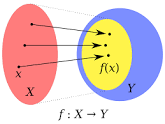
A surjective function (also known as surjection, or onto function) is a function f such that for every element y from the codomain of f there exists an input element x such that f(x) = y.
A bijective function f : X → Y is a one-to-one (injective) and onto (surjective) mapping of a set X to a set Y
Linear Transformations
Now we turn our attention to functions or transformations of vector spaces that do not “mess up” vector addition and scalar multiplication.- \( T({\bf x} + {\bf y}) = T({\bf x}) + T({\bf y}) \) (Additivity property),
- \( T( \alpha\,{\bf x} ) = \alpha\,T( {\bf x} ) \) (Homogeneity property).
- Let V = ℝ≤n[x] be a space of polynomials in variable x with real coefficients of degree no larger than n. Let U = ℝ≤n−1[x] be a similar space of polynomials but with degree up to n−1. We consider the differential operator \( \displaystyle \texttt{D} :\, V \mapsto U \) that is defined by \( \displaystyle \texttt{D}\,p(x) = p'(x) . \) As you know from calculus, this differential operator is linear.
-
Let V = ℝ≤1[x] be a space of polynomials in variable x with real coefficients of degree 1, and U = ℝ≤2[x]. For any polynomial p(x) = 𝑎x + b ∈ V, we assign another polynomial T(𝑎x + b) = (½)𝑎x² + bx ∈ U.
This transformation T : V ⇾ U is linear because \begin{align*} T \left( ax +b + cx +d \right) &= T \left( (a+c)\,x +b + d \right) \\ &= \frac{1}{2} \left( a + b \right) x^2 + \left( b + d \right) x \\ &= T \left( ax +b \right) + T \left( cx +d \right) , \end{align*} and for any real number λ, we have \begin{align*} T \left( \lambda \left( ax +b \right) \right) &= T \left( \lambda ax + \lambda b \right) \\ &= \frac{1}{2}\, \lambda a\,x^2 + \lambda b\,x = \lambda T \left( ax +b \right) . \end{align*}
- Let V = ℭ[0, 1] be a space of all continuous real-valued functions on interval [0, 1]. We define a linear transformation φ : V ⇾ ℝ by \[ \varphi (f) = \int_0^1 f(x)\,{\text d} x . \qquad \forall f \in V. \] This linear transformation is known as a functional on V.
- Let V = ℝ3,2 be the space of all 3×2 matrices with real entries. We define a linear operator A : V ⇾ V by \[ A\,\begin{bmatrix} a & b \\ c & d \\ e & f \end{bmatrix} = \begin{bmatrix} 1 & 2 & 3 \\ 4 & 5 & 6 \\ 7 & 8 & 9 \end{bmatrix} \, \begin{bmatrix} a & b \\ c & d \\ e & f \end{bmatrix} , \] where it is understood that two matrices are multiplied: \[ \begin{bmatrix} 1 & 2 & 3 \\ 4 & 5 & 6 \\ 7 & 8 & 9 \end{bmatrix} \, \begin{bmatrix} a & b \\ c & d \\ e & f \end{bmatrix} = \begin{bmatrix} a + 2c + 3 e & b + 2 d + 3 f \\ 4a + 5 c + 6 e & 4 b + 5 d + 6 f \\ 7a + 8c + 9e & 7b +8 d + 9f \end{bmatrix} \] So multiplication by a 3 × 3 mutrix we generate a linear transformation in the vector space of matrices ℝ3,2.
- Let us consider a vector space of square matrices with real coefficients: ℝn,n. For any matrix A ∈ ℝn,n, we define a linear transformation \[ T \left( {\bf A} \right) = {\bf A}^{\mathrm{T}} , \] where "T" means transposition (swap rows and columns).
In above discussion, we never used specific knowledge that T acts from ℝ into ℝ. Therefore the same conclusion about the form of linear transformation is valid for any transformation in the filed of rational numbers ℚ ⇾ ℚ or in the field of complex numbers ℂ ⇾ ℂ.
We summarize the almost obvious statements about linear transformation in the following proposition.
Theorem 1: Let V and U be a vector spaces and T : V ⇾ U be linear transformation.
- If T is a linear transformation, then T(0) = 0.
- T is a linear transformation if and only if for any \( {\bf x}_1 , \ldots , {\bf x}_n \in V \) and any real or complex scalars \( a_1 , \ldots , a_n \)
Corollary 1: For any two vector spaces V and U over the same field 𝔽, the set of all linear transformations from V to U, denoted by ℒ(V, U), is a vector space with addition and scalar multiplication defined as follows \[ \left( S + T \right) ({\bf v}) = S({\bf v}) + T({\bf v}), \qquad \alpha\,T(({\bf v}) = T(\alpha{\bf v}) . \]
Matrix as a linear transformations
Every n × n matrix A ∈ 𝔽n×m can be considered as a linear operator maping 𝔽n into 𝔽m.Similarly, an m × n -matrix A ∈ 𝔽
Since every column vector space 𝔽n×1 is isomorphic to the direct product space 𝔽n, matrix A defines a linear transformation, which we denote as TA. In our case, we obtain \[ T_A \, : \mathbb{F}^3 \,\mapsto\, \mathbb{F}^2 , \qquad T_A (x, y, z) = (3x + 2y + z, -x + 2y -3z ) . \]
Similarly, when matrix A is considered as an operator acting from the right, we have \[ \left[ u, v \right] \, \begin{bmatrix} \phantom{-}3 & 2 & \phantom{-}1 \\ -1 & 2 & -3 \end{bmatrix} = \begin{bmatrix} 3u - v & 2 u + 2v & u - 3v \end{bmatrix} \in \mathbb{F}^{1 \times 3} . \] When matrix A acts from right, it generates a linear transformation TA : 𝔽2 ⇾ 𝔽3 as \[ T_A (u, v) = (3u - v , 2 u + 2v , u - 3v) . \]
As a rule, we will consider action of matrices on vectors from the left (similar to all European languages that wring words from left to right). This approach requires utilization of column vectors from vector space 𝔽n×1 rather than Cartesian product 𝔽n.
The matrix of a linear transformation
In fact, matrix transformations are not just an example of linear transformations, but they are essentially the only example. One of the central theorems in linear algebra is that all linear transformations T : 𝔽3×1 ⇾ 𝔽2×1 are in fact matrix transformations. Therefore, a matrix can be regarded as a notation for a linear transformation, and vice versa. This is the subject of the following theorem.To see this, let \[ {\bf v} = \begin{bmatrix} x_1 \\ x_2 \\ \vdots \\ x_n \end{bmatrix} \in \mathbb{F}^{n\times 1} , \] be some arbitrary element of 𝔽n×1. Then v = x1e1 + x2e2 + ⋯ + xnen, and we have: \begin{align*} T({\bf v}) &= T \left( x_1 {\bf e}_1 + x_2 {\bf e}_2 + \cdots + x_n {\bf e}_n \right) \\ &= T \left( x_1 {\bf e}_1 \right) + T \left( x_2 {\bf e}_2 \right) + \cdots + T \left( x_n {\bf e}_n \right) \\ &= x_1 T \left( {\bf e}_1 \right) + x_2 T \left( {\bf e}_2 \right) + \cdots + x_n T \left( {\bf e}_n \right) \\ &= x_1 {\vd u}_1 + x_2 {\vd u}_2 + \cdots + x_n {\vd u}_n \\ &= {\bf A}\,{\bf v} . \end{align*}
Using Eq.(3), we obtain \[ \left[ T \right] = {\bf A} = \begin{bmatrix} \phantom{-}2 & 1 & 2 \\ -1 & 1 & 3 \end{bmatrix} . \]
In summary, the matrix corresponding to the linear transformation T has as its columns the vectors T(e1), T(e2), … , T(en), i.e., the images of the standard basis vectors. We can visualize this matrix as follows:
Corollary 2: Suppose V = 𝔽n and U = 𝔽m are vector spaces. As vector space over 𝔽, the space of all linear transformations ℒ(V, U) is isomorphic to the space of matrices of dimension m × n, so ℒ(𝔽m, 𝔽n) ≌ 𝔽m×n.
In order to find the matrix of this linear transformation, we compute the images of the standard basis vectors: \[ T({\bf e}_1 ) = T \left( \begin{bmatrix} 1 \\ 0 \end{bmatrix} \right) = \begin{bmatrix} \phantom{-}2 \\ -1 \\ \phantom{-}5 \end{bmatrix} , \qquad T({\bf e}_2 ) = T \left( \begin{bmatrix} 0 \\ 1 \end{bmatrix} \right) = \begin{bmatrix} -1 \\ \phantom{-}1 \\ -3 \end{bmatrix} . \] The matrix A = [T] has T(e₁) and T(e₂) as its columns. Therefore, \[ {\bf A} = \left] T \right] = \begin{bmatrix} \phantom{-}2 & -1 \\ -1 & \phantom{-}1 \\ \phantom{-}5 & -3 \end{bmatrix} \]
To find the matrix of T, we must compute the images of the standard basis vectors T(e₁), T(e₂) and T(e₃). This yields \begin{align*} T \left( {\bf e}_1 \right) &= \mbox{prof}_{\bf u} ({\bf e}_1 ) = \frac{{\bf u} \bullet {\bf e}_1}{\| {\bf u} \|^2}\,{\bf u} = \frac{1}{14} \begin{bmatrix} \phantom{-}1 \\ -2 \\ \phantom{-}3 \end{bmatrix} , \\ T \left( {\bf e}_2 \right) &= \mbox{prof}_{\bf u} ({\bf e}_2 ) = \frac{{\bf u} \bullet {\bf e}_2}{\| {\bf u} \|^2}\,{\bf u} = \frac{-2}{14} \begin{bmatrix} \phantom{-}1 \\ -2 \\ \phantom{-}3 \end{bmatrix} , \\ T \left( {\bf e}_3 \right) &= \mbox{prof}_{\bf u} ({\bf e}_3 ) = \frac{{\bf u} \bullet {\bf e}_3}{\| {\bf u} \|^2}\,{\bf u} = \frac{3}{14} \begin{bmatrix} \phantom{-}1 \\ -2 \\ \phantom{-}3 \end{bmatrix} , \end{align*} because ∥ u ∥² = 14. Hence the matrix of T is \[ \left[ T \right] = \frac{1}{14} \begin{bmatrix} 1 & -2 & 3 \\ -2 & 4 & -6 \\ 3 & -6 & 9\end{bmatrix} , \] which is rank 1.
MatrixRank[A]
Composition of Transformations
Simplify[5*y1 - 4*y2 + 3*y3 - 2*y4]
- In order for S ∘ T to be defined, the codomain of T must equal the domain of S.
- The domain of S ∘ T is the domain of T.
- The codomain of S ∘ T is the codomain of S.
Let C be the standard matrix of S ∘ T; so we have T(x) = A x, S(y) = B y, and S ∘ T(x) = C x. According to Theorem 3, the first column of C is C e₁, and the first column of B is B e₁. We have \[ S \circ T ({\bf e}_1 ) = S \left( T \left( {\bf e}_1 \right) \right) = S \left( {\bf B\,e}_1 \right) = {\bf A} \left( {\bf B\,e}_1 \right) . \] By definition, the first column of the product A B is the product of A with the first column of B, which is B e₁, so \[ {\bf C}\,{\bf e}_1 = S \circ T({\bf e}_1 ) = S \left( T \left( {\bf e}_1 \right) \right) = S \left( {\bf B}\,{\bf e}_1 \right) = \left( {\bf A\,B} \right) {\bf e}_1 . \] It follows that C has the same first column as A B. The same argument as applied to the i-th standard coordinate vector ei shows that C and A B have the same i-th column; since they have the same columns, they are the same matrix.
B = {{5, -4, 3, -2}, {3, 1, -3, -4}, {1, -2, -4, 1}}
B.A
Homogeneous coordinates have a natural application to Computer Graphics; they form a basis for the projective geometry used extensively to project a three-dimensional scene onto a two- dimensional image plane. They also unify the treatment of common graphical transformations and operations. Homogeneous coordinates are also used in the related areas of CAD/CAM [Zeid], robotics, computational projective geometry, and fixed point arithmetic.
The homogeneous coordinate system is formed by equating each vector in ℝ² with a vector in ℝ³ having the same first two coordinates and having 1 as its third coordinate. \[ \left[ \begin{array}{c} x_1 \\ x_2 \end{array} \right] \, \longleftrightarrow \, \left[ \begin{array}{c} x_1 \\ x_2 \\ 1 \end{array} \right] . \] When we want to plot a point represented by the homogeneous coordinate vector (x₁, x₂, 1), we simply ignore the third coordinate and plot the ordered pair (x₁, x₂).
One of the advantages of homogeneous coordinates is that they allow for an easy combination of multiple transformations by concatenating several matrix-vector multiplications.
If the homogeneous coordinates of a point are multiplied by a non-zero scalar, then the resulting coordinates represent the same point. For example, the point (1, 2) in Cartesian coordinates has the following same homogeneous coordinates as \[ (1, 2 ) \qquad \iff \qquad \begin{split} (1, 2, 1) \\ (2, 4, 2) \\ (100, 200, 100) . \end{split} \]
The linear transformations discussed earlier must now be represented by 3 × 3 matrices. To do this, we take the 2 × 2 matrix representation and augment it by attaching the third row and third column of the 3 × 3 identity matrix. For example, in place of the 2 × 2 dilation matrix \[ \begin{bmatrix} 2 & 0 \\ 0 & 3 \end{bmatrix} , \] we have the 3 × 3 matrix \[ \begin{bmatrix} 2 & 0 & 0 \\ 0 & 3 & 0 \\ 0 & 0 & 1 \end{bmatrix} , \] Note that scaling gives \[ \begin{bmatrix} 2 & 0 & 0 \\ 0 & 3 & 0 \\ 0 & 0 & 1 \end{bmatrix} \left[ \begin{array}{c} x_1 \\ x_2 \\ 1 \end{array} \right] = \left[ \begin{array}{c} 2\,x_1 \\ 3\,x_3 \\ 1 \end{array} \right] \quad\mbox{and} \quad \begin{bmatrix} 2 & 0 \\ 0 & 3 \end{bmatrix} \left[ \begin{array}{c} x_1 \\ x_2 \end{array} \right] = \left[ \begin{array}{c} 2\,x_1 \\ 3\,x_2 \end{array} \right] \] Rotation operation is performed as \[ \begin{bmatrix} \cos\theta & -\sin\theta & 0 \\ \sin\theta & \cos\theta & 0 \\ 0 & 0 & 1 \end{bmatrix} \left[ \begin{array}{c} x_1 \\ x_2 \\ 1 \end{array} \right] = \left[ \begin{array}{c} x_1 \cos\theta-x_2 \sin\theta \\ x_1 \sin\theta + x_2 \cos\theta \\ 1 \end{array} \right] \qquad\mbox{and} \qquad \begin{bmatrix} \cos\theta & -\sin\theta \\ \sin\theta & \cos\theta \end{bmatrix} \left[ \begin{array}{c} x_1 \\ x_2 \end{array} \right] = \left[ \begin{array}{c} x_1 \cos\theta - x_2 \sin\theta \\ x_1 \sin\theta + x_2 \cos\theta \end{array} \right] \] Translation in homogeneous coordinates: \[ \begin{bmatrix} 1 & 0 & a \\ 0 & 1 & b \\ 0 & 0 & 1 \end{bmatrix} \left[ \begin{array}{c} x_1 \\ x_2 \\ 1 \end{array} \right] = \left[ \begin{array}{c} x_1 \\ x_2 \\ 1 \end{array} \right] + \left[ \begin{array}{c} a \\ b \\ 1 \end{array} \right] . \] So now in homogeneous coordinates, we are able to do scaling, rotation and translation by simple matrix multiplication instead of applying all the transformations separately, which is much more convenient for us when we want to combine these operations together.
In order to convert from homogeneous coordinates (x, y, w) to Cartesian coordinates, we simply divide x and y by w;
\[
(x, y, w) \qquad \iff \qquad \left( \frac{x}{w} , \frac{y}{w} , 1 \right) \qquad \iff \qquad \left( \frac{x}{w} , \frac{y}{w}\right) .
\]
- Hu, Yasen, Homogeneous Coordinates.
- Leon, S.J., de Pillis, L., Linear Algebra with Applications, Pearson, Harlow, ISBN 13: 978-1-292-35486-6
- Wikipedia.
Figure 16.1 below shows the initial position of a model airplane and four basic fources acting on it. In describing yaw, pitch, and roll, the current coordinate system is given in terms of the position of the vehicle. It is always assumed that the craft is situated on the xy-plane with its nose pointing in the direction of the positive x-axis and the left wing pointing in the direction of the positive y-axis. Furthermore, when the plane moves, the three coordinate axes move with the vehicle.

|

|
A force may be thought of as a push or pull in a specific direction. This slide shows the forces that act on an airplane in flight.
A yaw is a rotation in the xy-plane. Figure 16.3 illustrates a yaw of 15°. In this case, the craft has been rotated 15° to the right (clockwise). Viewed as a linear transformation in 3-space, a yaw is simply a rotation about the z-axis. Note that if the initial coordinates of the nose of the model plane are represented by the vector (1, 0, 0), then its xyz coordinates after the yaw transformation will still be (1, 0, 0), since the coordinate axis rotated with the craft. In the initial position of the airplane, the x, y, and z axes are in the same directions as the front-back, left-right, and top-bottom axes shown in the figure. We will refer to this initial front, left, top axis system as the FLT axis system. After the 30° yaw, the position of the nose of the craft with respect to the FLT axis system is \( \displaystyle \left( \frac{\sqrt{3}}{2}, - \frac{1}{2} , 0 \right) . \)

|

|
If we view a yaw transformation L in terms of the FLT axis system, it is easy to find a matrix representation. If T corresponds to yaw by an angle θ, then T will rotate the points (1, 0, 0) and (0, 1, 0) to the positions (cosθ, − sinθ, 0) and (sinθ, cosθ, 0), respectively. The point (0, 0, 1) will remained unchanged by the yaw since it is on the axis of rotation. In terms of column vectors, if y₁, y₂, and y₃ are the images of the standard basis vectors for ℝ³ under T, then \[ {\bf y}_1 = T\left( {\bf e}_1 \right) = \left[ \begin{array}{c} \cos\theta \\ -\sin\theta \\ 0 \end{array} \right] , \qquad {\bf y}_2 = T\left( {\bf e}_2 \right) = \left[ \begin{array}{c} \sin\theta \\ \cos\theta \\ 0 \end{array} \right] , \qquad {\bf y}_3 = T\left( {\bf e}_3 \right) = \left[ \begin{array}{c} 0 \\ 0 \\ 1 \end{array} \right] . \] Therefore, the matrix representation of the yaw transformation becomes \[ {\bf Y} = \begin{bmatrix} \cos\theta & \sin\theta & 0 \\ -\sin\theta & \cos\theta & 0 \\ 0 & 0 & 1 \end{bmatrix} . \]

|

|
A pitch is a rotation of the aircraft in the xz-plane. Figure 4.2.5(c) illustrates a pitch of −30°. Since the angle is negative, the nose of the aircraft is rotated 30&de; downward, toward the bottom axis of the figure. Viewed as a linear transformation in 3-space, a pitch is simply a rotation about the y-axis. As with the yaw, we can find the matrix for a pitch transformation with respect to the FLT axis system. If T is a pitch transformation with angle of rotation φ, the matrix representation of T is given by \[ {\bf P} = \begin{bmatrix} \cos\varphi & 0 & -\sin\varphi \\ 0 & 1 & 0 \\ \sin\varphi & 0 & \cos\varphi \end{bmatrix} . \]

|

|
A roll is a rotation of the aircraft in the yz-plane. Figure 4.2.5(d) illustrates a roll of 30°. In this case, the left wing is rotated up 30° toward the top axis in the figure and the right wing is rotated 30° downward toward the bottom axis. Viewed as a linear transformation in 3-space, a roll is simply a rotation about the x-axis. As with the yaw and pitch, we can find the matrix representation for a roll transformation with respect to the FLT axis system. If T is a roll transformation with angle of rotation ψ, the matrix representation of L is given by \[ {\bf R} = \begin{bmatrix} 1 & 0 & 0 \\ 0 & \cos\psi & -\sin\psi \\ 0 & \sin\psi & \cos\psi \end{bmatrix} . \]
If we perform a yaw by an angle θ and then a pitch by an angle φ, the composite transformation is linear; however, its matrix representation is not equal to the product P Y. The effect of the yaw on the standard basis vectors e₁, e₂, and e₃ is to rotate them to the new directions y₁, y₂, and yy₃. So the vectors y₁, y₂, and yy₃ will define the directions of the x, y, and z axes when we do the pitch. The desired pitch transformation is then a rotation about the new y-axis (i.e., the axis in the direction of the vector y₂). The vectors y₁ and y₃ form a plane, and when the pitch is applied, they are both rotated by an angle φ in that plane. The vector y₂ will remain unaffected by the pitch, since it lies on the axis of rotation. Thus, the composite transformation T has the following effect on the standard basis vectors: \begin{align*} {\bf e}_1 & \stackrel{\mbox{yaw}}{\longrightarrow} \,{\bf y}_1 \, \stackrel{\mbox{pitch}}{\longrightarrow} \,\cos\varphi \,{\bf y}_1 + \sin\varphi \,{\bf y}_3 , \\ {\bf e}_2 & \stackrel{\mbox{yaw}}{\longrightarrow} \,{\bf y}_2 \, \stackrel{\mbox{pitch}}{\longrightarrow} \,{\bf y}_2 , \\ {\bf e}_3 & \stackrel{\mbox{yaw}}{\longrightarrow} \,{\bf y}_1 \, \stackrel{\mbox{pitch}}{\longrightarrow} \,\sin\varphi \,{\bf y}_1 + \cos\varphi \, {\bf y}_3 . \end{align*}
The images of the standard basis vectors form the columns of the matrix representing the composite transformation: \[ \left( \cos\varphi \,{\bf y}_1 + \sin \varphi \,{\bf y}_3 , {\bf y}_2 , -\sin\varphi \,{\bf y}_1 + \cos \varphi \,{\bf y}_3 \right) = \left( {\bf y}_1 , {\bf y}_2 , {\bf y}_3 \right) \begin{bmatrix} \cos \varphi & 0 & - \sin \varphi \\ 0 & 1 & 0 \\ \sin\varphi & 0 & \cos \varphi \end{bmatrix} . \]
It follows that matrix representation of the composite is a product of the two individual matrices representing the yaw and the pitch, but the product must be taken in the reverse order, with the yaw matrix Y on the left and the pitch matrix P on the right. Similarly, for a composite transformation of a yaw with angle θ, followed by a pitch with angle φ, and then a roll with angle ψ, the matrix representation of the composite transformation would be the product Y P R.
- Let u ∈ 𝔽n be a fixed non-zero vector. The function T defined by T(v) = v + u has the effect of translating all vectors by adding u. Show that T is not a linear transformation.
- Which of the following vector functions are linear transformations? \[ T_1 \left( \begin{bmatrix} x \\ y \end{bmatrix} \right) = \begin{bmatrix} x \left( y + z \right) \\ x-2y \\ z+ x \end{bmatrix} , \qquad T_2 \left( \begin{bmatrix} x \\ y \end{bmatrix} \right) = \begin{bmatrix} x + y^2 \\ y\left( x-2z \right) \\ 3z \end{bmatrix} . \]
- Consider the following functions T : ℝ³ ⇾ ℝ². Explain why each of these functions T is not linear. \[ \mbox{(a)}\quad T \left( \begin{bmatrix} x \\ y \\ z \end{bmatrix} \right) = \begin{bmatrix} 3x -z+2 \\ y-z \end{bmatrix} , \qquad \mbox{(b)}\quad T \left( \begin{bmatrix} x \\ y \\ z \end{bmatrix} \right) = \begin{bmatrix} x^2 + 2y \\ z-y \end{bmatrix} \]
- Find the matrix corresponding to the given transformation \[ \mbox{(a)}\quad \begin{bmatrix} x_{1} \\ x_{2} \\ \end{bmatrix} \,\mapsto \, \begin{bmatrix} 3x_{1}-4x_{2}\\ 8x_{1}+15x_{2}\\ \end{bmatrix} ; \qquad \mbox{(b)}\quad \begin{bmatrix} x_{1} \\ x_{2} \\ x_{3} \\ \end{bmatrix} \,\mapsto \, \begin{bmatrix} x_{1}-3x_{2}+2x_{3}\\ 0 \\ 2x_{1}-x_{3} \\ -x_{1}+4x_{2}-3x_{3} \\ \end{bmatrix} ; \] \[ \mbox{(c)}\quad \begin{bmatrix} x_{1} \\ x_{2} \\ x_{3} \\ \end{bmatrix} \,\mapsto \, \begin{bmatrix} 4x_{1}\\ 7x_{2} \\ -8x_{3} \\ \end{bmatrix} ; \qquad \mbox{(d)}\quad \begin{bmatrix} x_{1} \\ x_{2} \\ x_{3} \\ \end{bmatrix} \,\mapsto \, \begin{bmatrix} 8x_{1}+4x_{2}-x_{3}\\ 10x_{1}-9x_{2}+12x_{13} \\ -2x_{1}-x_{3} \\ \end{bmatrix}; \] \[ \mbox{(e)}\quad \begin{bmatrix} x_{1} \\ x_{2} \\ x_{3} \\ x_{4} \\ \end{bmatrix} \,\mapsto \, \begin{bmatrix} 2x_{1}+2x_{3}-2x_{4}\\ -x_{4} \\ 2x_{1}-1x_{3} \\ -x_{2}+3x_{4} \\ \end{bmatrix}; \qquad \mbox{(f)}\quad \]
- Does the transformation satisfy the property T(A + B) = T(A) + T(B) ? \[ \mbox{(a)}\quad \begin{bmatrix} x_{1} \\ x_{2} \\ \end{bmatrix} \,\mapsto \, \begin{bmatrix} x_{1}+2\\ x_{2}+2 \\ \end{bmatrix}; \qquad \mbox{(b)}\quad \begin{bmatrix} x_{1} \\ x_{2} \\ \end{bmatrix} \,\mapsto \, \begin{bmatrix} 2x_{1} \\ 3x_{2} \\ \end{bmatrix}. \]
- Does the transformation satisfy the property T(cA) = cT(A) for a constant c ? \[ \mbox{(a)}\quad \begin{bmatrix} x_{1} \\ x_{2} \\ \end{bmatrix} \,\mapsto \, \begin{bmatrix} x_{1}+2x_{2} \\ 3x_{2} \end{bmatrix}; \qquad \mbox{(b)}\quad \begin{bmatrix} x_{1} \\ x_{2} \end{bmatrix} \,\mapsto \, \begin{bmatrix} x_{1}^2 \\ x_{2} \end{bmatrix}. \]
- Are the following transformations linear? Check that both properties T(A + B) = T(A) + T(B) and T(cA) = cT(A) are satisfied. \[ \mbox{(a)}\quad \begin{bmatrix} x_{1} \\ x_{2} \\ x_{3} \\ \end{bmatrix} \,\mapsto \, \begin{bmatrix} 4x_{1}+x_{3}\\ -2x_{1}+3x_{2} \end{bmatrix} ; \qquad \mbox{(b)}\quad \begin{bmatrix} x_{1} \\ x_{2} \\ x_{3} \\ \end{bmatrix} \,\mapsto \, \begin{bmatrix} 4+ 2x_{1}+x_{3}\\ x_{1}+3x_{2} \end{bmatrix} . \]
-
Find the composition of transformations S with T, i.e.
S∘T.
- \[ \quad S:\ \begin{bmatrix} x_{1} \\ x_{2} \\ \end{bmatrix} \,\mapsto \, \begin{bmatrix} x_{1}-4x_{2} \\ 6x_{1}+3x_{2} \\ -2x_{1}+4x_{2} \end{bmatrix}, \quad T:\ \begin{bmatrix} x_{1} \\ x_{2} \\ x_{3} \\ \end{bmatrix} \,\mapsto \, \begin{bmatrix} 3x_{1}-2x_{2}+x_{3} \\ 5x_{1}+2x_{2}-7x_{3} \\ 1x_{1}+7x_{2}-4x_{3} \\ \end{bmatrix} \]
- \[ \quad S:\ \begin{bmatrix} x_{1} \\ x_{2} \\ x_{3} \\ x_{4} \\ \end{bmatrix} \,\mapsto \, \begin{bmatrix} 6x_{1}+3x_{2}-x_{3} \\ x_{1}+x_{2}+x_{3}+4x_{4} \\ -2x_{1}+5x_{2}+2x_{4} \\ \end{bmatrix}, \quad T\,:\, \begin{bmatrix} x_{1} \\ x_{2} \\ x_{3} \\ \end{bmatrix} \,\mapsto \, \begin{bmatrix} 2x_{1}+x_{2}+4x_{3} \\ x_{2}+x_{3}\\ \end{bmatrix}; \]
- \[ \quad S:\ \begin{bmatrix} x_{1} \\ x_{2} \\ \end{bmatrix} \,\mapsto \, \begin{bmatrix} x_{1}+2x_{2} \\ 4x_{1}+3x_{2} \\ 2x_{1}+4x_{2} \\ \end{bmatrix}, \quad T: \ \begin{bmatrix} x_{1} \\ x_{2} \\ x_{3} \\ \end{bmatrix} \,\mapsto \, \begin{bmatrix} 1x_{1}-2x_{2}+3x_{3} \\ 3x_{1}-2x_{2}+x_{3} \\ 2x_{1}+x_{2}-3x_{3} \end{bmatrix}. \]
- Let T be a linear transformation from ℝ³ into ℝ² defined by relations T(i) = (1,2), T(j) = (3,-4), and T(k) = (-5,6). Find the standard matrix for T.
- Let T : ℝ² ⇾ ℝ² be a linear transformation. If T(1, 2) = (2, −3) and T(3, −4) = (4, 1), find the value of T(5, 7).
-
Determine whether the following are linear transformations from ℝ³ into ℝ²
- T(x) = (x₂, x₁);
- T(x) = (0, 0);
- T(x) = (x₂ + 1, x₁ −1);, x₁x₃).
- T(x) = (x₁ + x₃
-
Determine whether the following are linear transformations from ℝ² into ℝ³
- T(x) = (0, 0, x₁);
- T(x) = (0, 0, 1);
- T(x) = (x₁, x₂, x₁);
- T(x) = (x₁ + x₂, x₁ − x₂, x₁).
-
Determine whether the following are linear operators on ℝn×n:
- T(A) = 3A;
- T(A) = A − I;
- T(A) = A − AT;
- T(A) = AAT − ATA.
-
Let C be a fixed n × n matrix. Determine whether the
following are linear operators on ℝn×n:
- T(A) = CA − AC;
- T(A) = C²A;
- T(A) = A²C.
-
For each of the following vector functions T : ℝn ⇾ ℝn, show that T is a linear transformation and find the corresponding matrix A = [T] such that TA(v) = Av.
- T multiplies the j-th component of v by a non-zero number b.
- T adds b times the j-th component of v to the i-th component.
- T switches the i-th and j-th components.
- Ch.G. Cullen, "Matrices and linear transformations" , Dover, reprint (1990) pp. 236ff
- Leon, S.J., de Pillis, L., Linear Algebra with Applications, Pearson, Harlow, ISBN 13: 978-1-292-35486-6