This section presents applications of Legendre polynomials for solving Laplace's equation in spherical coordinates.
Let us introduce in ℝ³
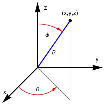
spherical coordinates :
\[
\begin{split}
x &= \rho\,\cos \phi\,\sin\theta , \\
y &= \rho\,\sin \phi\,\sin\theta , \\
z &= \rho\,\cos\theta ;
\end{split} \qquad \Longrightarrow \qquad \phi = \begin{cases}
\arctan \left( y/x \right) , & \ \mbox{ if} \quad x > 0 , \\
\arctan \left( y/x \right) + \pi , & \ \mbox{ if} \quad x < 0 , \\
\frac{\pi}{2} , & \ \mbox{ else}.
\end{cases} .
\]
As usual, the location of a point (
x, y, z ) is specified by the distance ρ of the point from the origin, the angle ϕ between the position vector and the
z -axis, the polar angle measured down from the north pole, and the azimuthal angleq θ from the
x -axis to the projection of the position vector onto the
xy plane, analogous to longitude in earth measuring coordinates:
\[
\rho = \sqrt{x^2 + y^2 + z^2} \ge 0 \qquad\mbox{and} \qquad \theta = \mbox{arccos} \frac{z}{\rho} , \qquad 0 \le \theta < 2\pi , \quad 0 \le \phi \le \pi .
\]
az = Graphics[{Black, Thickness[0.01], Arrowheads[0.1],
Arrow[{{0, 0}, {0, 1.2}}]}];
Spherical coordinates.
Mathematica code
The Laplace's equation Δu = 0 in spherical coordinates (ρ θ ϕ) can be written as
\begin{equation} \label{EqSphere.1}
\nabla^2 u = \frac{1}{\rho^2} \,\frac{\partial}{\partial \rho} \left( \rho^2 \frac{\partial u}{\partial \rho} \right) + \frac{1}{\rho^2 \sin \phi} \,\frac{\partial}{\partial \phi} \left( \sin\phi \,\frac{\partial u}{\partial\phi} \right) + \frac{1}{\rho^2 \sin^2 \phi} \,\frac{\partial^2 u}{\partial \theta^2} = 0.
\end{equation}
We look for partial nontrivial (not identically zero) solutions of equation \eqref{EqSphere.1} that is represented as a product of two functions
\[
u(\rho , \theta , \phi ) = R(\rho )\, Y(\theta , \phi ) .
\]
Substituting this product-function into Eq.\eqref{EqSphere.1} and divide the result by
u , we obtain
\[
\frac{1}{R(\rho )} \,\frac{\partial}{\partial \rho} \left( \rho^2 \frac{\partial R}{\partial \rho} \right) + \frac{1}{Y(\theta , \phi )} \left[ \frac{1}{\sin \phi} \,\frac{\partial}{\partial \phi} \left( \sin\phi \,\frac{\partial Y}{\partial\phi} \right) + \frac{1}{\sin^2 \phi} \,\frac{\partial^2 Y}{\partial \theta^2} \right] = 0.
\]
The first term in the left-hand side does not depend on angles (θ, ϕ). Therefore, the equation is valid only when every term is a constant:
\[
\frac{1}{R(\rho )} \,\frac{\partial}{\partial \rho} \left( \rho^2 \frac{\partial R}{\partial \rho} \right) = \lambda ,
\]
and
\[
\frac{1}{Y(\theta , \phi )} \left[ \frac{1}{\sin \phi} \,\frac{\partial}{\partial \phi} \left( \sin\phi \,\frac{\partial Y}{\partial\phi} \right) + \frac{1}{\sin^2 \phi} \,\frac{\partial^2 Y}{\partial \theta^2} \right] = -\lambda ,
\]
where λ is a constant. From these equations, it follows
\begin{equation} \label{EqSphere.2}
\rho^2 \frac{{\text d}^2 R}{{\text d}\rho^2} + 2\rho\,\frac{{\text d}R}{{\text d}\rho} - \lambda\,R(\rho ) = 0,
\end{equation}
and
\begin{equation} \label{EqSphere.3}
\frac{1}{\sin \phi} \,\frac{\partial}{\partial \phi} \left( \sin\phi \,\frac{\partial Y}{\partial\phi} \right) + \frac{1}{\sin^2 \phi} \,\frac{\partial^2 Y}{\partial \theta^2} + \lambda\, Y(\theta , \phi ) = 0.
\end{equation}
Eq.\eqref{EqSphere.3} can also be solved by separation of variables
Y (θ, ϕ) = Θ(θ) Φ(ϕ), which leads to
\[
\frac{\Theta (\theta )}{\sin \phi} \,\frac{{\text d}}{{\text d} \phi} \left( \sin\phi \,\frac{{\text d}\Phi}{{\text d}\phi} \right) + \frac{\Phi (\phi )}{\sin^2 \phi} \,\frac{{\text d}^2 \Theta}{{\text d} \theta^2} + \lambda\, \Theta (\theta )\, \Phi(\phi ) = 0 \qquad \Longrightarrow \qquad - \lambda\,\sin^2 \phi - \frac{\sin\phi}{\Phi (\phi )} \,\frac{{\text d}}{{\text d} \phi} \left( \sin\phi \,\frac{{\text d}\Phi}{{\text d}\phi} \right) = \frac{1}{\Theta (\theta )} \,\frac{{\text d}^2 \Theta}{{\text d} \theta^2} .
\]
Since we separate variables, we get two equations
\[
\frac{1}{\Theta (\theta )} \,\frac{{\text d}^2 \Theta}{{\text d} \theta^2} = -\mu \qquad \Longrightarrow \qquad \frac{{\text d}^2 \Theta}{{\text d} \theta^2} + \mu \,\Theta (\theta ) = 0
\]
and
\[
\lambda\,\sin^2 \phi + \frac{\sin\phi}{\Phi (\phi )} \,\frac{{\text d}}{{\text d} \phi} \left( \sin\phi \,\frac{{\text d}\Phi}{{\text d}\phi} \right) = \mu \qquad \Longrightarrow \qquad \sin\phi\,\frac{{\text d}}{{\text d} \phi} \left( \sin\phi \,\frac{{\text d}\Phi}{{\text d}\phi} \right) - \left( \mu - \lambda\,\sin^2 \phi \right) \Phi (\phi ) = 0 .
\]
From the latter, we get a Sturm--Liouville problem
\[
\frac{{\text d}^2 \Theta}{{\text d} \theta^2} + \mu \,\Theta (\theta ) = 0 , \qquad \Theta (\theta ) = \Theta (\theta + 2 \pi ) ,
\]
with eigenvalues μ =
m ², for which correspond eigenfunctions are
\[
\Theta_m (\theta ) = a_m \cos m\theta + b_m \sin m\theta , \qquad m=0,1,2,\ldots .
\]
Here 𝑎
m and
b m are some real constants.
Substuting this value μ =
m ² into equation for Φ, we get the Sturm--Liouville problem
\[
\sin\phi\,\frac{{\text d}}{{\text d} \phi} \left( \sin\phi \,\frac{{\text d}\Phi}{{\text d}\phi} \right) + \left( \lambda\,\sin^2 \phi - m^2 \right) \Phi (\phi ) = 0, \qquad \Phi (0) < \infty , \quad \Phi (\pi ) < \infty .
\]
Upon making substitution
x = cos(ϕ) and dividing by sin²(ϕ), we obtain a familiar
Sturm--Liouville problem
\[
\frac{\text d}{{\text d}x} \left( 1 - x^2 \right) \frac{{\text d}P(x)}{{\text d}x} + \left( \lambda - \frac{m^2}{1-x^2} \right) P(x) = 0 , \qquad P(-1) < \infty , \quad P(1) < \infty .
\]
The latter is a Sturm--Liouville problem for the
associated Legendre polynomials and we find eigenvalues and corresponding eigenfunctions:
\[
\lambda_n = n(n+1) , \qquad P(x) = P_{n,m} (x) = P_n^m (x) , \qquad n=0,1,2,\ldots ,
\]
where
P n,m (
x ), also denoted by
P n m (
x ), are the associated Legendre polynomials.
With this in hand, we determine eigenvalues and eigenfunctions for equation
\eqref{EqSphere.3}:
\begin{equation} \label{EqSphere.4}
Y_{n,m} (\theta , \phi ) = P_n^m (\cos\theta ) \left[ a_m \cos m\phi + b_m \sin m\phi \right] , \qquad m=0,1,2,\ldots , n, \quad n=0,1,2,\ldots .
\end{equation}
These functions
Y n,m (θ,
ϕ) are called
spherical functions . These functions are orthogonal
\begin{equation} \label{EqSphere.5}
\iint_{\Sigma}
Y_{n,m} (\theta , \phi )\, Y_{i,j} (\theta , \phi )\, \sin\theta\,{\text d}\theta\,{\text d}\phi = 0 \qquad\mbox{if} \quad m\ne i \quad \mbox{or} \quad m \ne j .
\end{equation}
Using
Mathematica , we find first ten spherical functions:
Series[1/Sqrt[1 - 2*x*t + t^2], {t, 0, 10}]
n
m
Spherical function
n = 0
m = 0
Y 0,0 (θ, ϕ) = 1
n = 1
m = 0
Y 1,0 (θ, ϕ) = cosθ
n = 1
m = 1
\( \displaystyle Y_{1,1} (\theta , \phi ) = -\sin \theta \left( a_1 \cos\phi + b_1 \sin\phi \right) \)
n = 2
m = 0
\( \displaystyle Y_{2,0} (\theta , \phi ) = \frac{1}{2} \left( 3 \cos^2 \theta -1 \right) \)
n = 2
m = 1
\( \displaystyle Y_{2,1} (\theta , \phi ) = -3\cos \theta\,\sin\theta \left[ a_1 \cos\phi + b_1 \sin\phi \right] \)
n = 2
m = 2
\( \displaystyle Y_{2,2} (\theta , \phi ) = 3\,\sin^2 \theta \left[ a_2 \cos 2\phi + b_2 \sin 2\phi \right] \)
n = 3
m = 0
\( \displaystyle Y_{3,0} (\theta , \phi ) = \frac{1}{2}\,\cos \theta \left( 5\cos^2 \theta - 3 \right) \)
n = 3
m = 1
\( \displaystyle Y_{3,1} (\theta , \phi ) = \frac{3}{2}\,\sin \theta \left( 1 - 5 \cos^2 \theta \right) \left[ a_1 \cos \phi + b_1 \sin \phi \right] \)
n = 3
m = 2
\( \displaystyle Y_{3,2} (\theta , \phi ) = 15\cos\theta \,\sin^2 \theta \left[ a_2 \cos 2\phi + b_2 \sin 2\phi \right] \)
n = 3
m = 3
\( \displaystyle Y_{3,3} (\theta , \phi ) = -15\,\sin^3 \theta \left[ a_3 \cos 3\phi + b_3 \sin 3\phi \right] \)
n = 4
m = 0
\( \displaystyle Y_{4,0} (\theta , \phi ) = \frac{1}{8} \left( 35\,\cos^4 \theta - 30\,\cos^2 \theta + 3 \right) \)
n = 4
m = 1
\( \displaystyle Y_{4,1} (\theta , \phi ) = \frac{5}{2}\,\cos \theta \,\sin\theta \left( 3 - 7 \cos^2 \theta \right) \left[ a_1 \cos \phi + b_1 \sin \phi \right] \)
n = 4
m = 2
\( \displaystyle Y_{4,2} (\theta , \phi ) = \frac{15}{2}\,\sin^2 \theta \left( 7\,\cos^2 \theta -1 \right) \left[ a_2 \cos 2\phi + b_2 \sin 2\phi \right] \)
n = 4
m = 3
\( \displaystyle Y_{4,3} (\theta , \phi ) = -105\,\cos\theta \,\sin^3 \theta \left[ a_3 \cos 3\phi + b_3 \sin 3\phi \right] \)
n = 4
m = 4
\( \displaystyle Y_{4,4} (\theta , \phi ) = 105\,\sin^4 \theta \left[ a_4 \cos 4\phi + b_4 \sin 4\phi \right] \)
n = 5
m = 0
\( \displaystyle Y_{5,0} (\theta , \phi ) = \frac{1}{8}\,\cos\theta \left( 63\,\cos^4 \theta - 70\,\cos^2 \theta + 15 \right) \)
Since Eq.\eqref{EqSphere.2} is an Eiler's ordinary differential equation , the
general solution of the radial equation becomes
\[
R(\rho ) = R_n (\rho ) = A_n \rho^{n} + B_n \rho^{-n-1} ,
\]
with some constants
A n and
B n . So partial nontrivial solutions of Laplace's equation are products of the radial solutions and spherical functions:
\( \displaystyle u_{n,m} (\rho , \theta , \phi ) = R_n (\rho )\, Y_{n,m} (\theta , \phi ) . \) Since Laplace's equation is homogeneous, any sum of these partial solutions will be also solutions of Laplace's equation. Hence, we seek the solution of
Laplace's equation as infinte sum:
\begin{equation} \label{EqSphere.6}
u(\rho , \theta , \phi ) = \sum_{n\ge 0} R_n (\rho ) \sum_{m=0}^n
Y_{n,m} (\theta , \phi ) = \sum_{n\ge 0} \left[ A_n \rho^{n} + B_n \rho^{-n-1} \right] \sum_{m=0}^n P_n^m (\cos\theta ) \left( a_m \cos m\phi + b_m \sin m\phi \right) .
\end{equation}
In particular, if we seek a solution in a domain not containing the origin, then its solution can be expressedthrough spherical functions as
\begin{equation} \label{EqSphere.7}
u(\rho , \theta , \phi ) = \sum_{n\ge 0} \left( \frac{R}{\rho} \right)^{n+1} \sum_{m=0}^n
Y_{n,m} (\theta , \phi ) = \sum_{n\ge 0} \left( \frac{R}{\rho} \right)^{n+1} \sum_{m=0}^n P_n^m (\cos\theta ) \left( a_m \cos m\phi + b_m \sin m\phi \right) .
\end{equation}
When we seek a harmonic function in a domain containing the origin, it solution becomes
\begin{equation} \label{EqSphere.8}
u(\rho , \theta , \phi ) = \sum_{n\ge 0} \left( \frac{\rho}{R} \right)^{n} \sum_{m=0}^n
Y_{n,m} (\theta , \phi ) = \sum_{n\ge 0} \left( \frac{\rho}{R} \right)^{n} \sum_{m=0}^n P_n^m (\cos\theta ) \left( a_m \cos m\phi + b_m \sin m\phi \right) .
\end{equation}
Example 1: Interior Dirichlet problem
Example 2: Outer Dirichlet problem
Example 3: Interior Neumann problem
Example 3:
\[
\nabla^2 u = 0 \quad (\rho < 3) , \qquad \left. \frac{\partial u}{\partial \rho} \right\vert_{\rho =3} = f(\theta , \phi ) .
\]
Example 4: Outer Neumann problem
Example 4:
\[
\nabla^2 u = 0 \quad (\rho > 2) , \qquad \left. \frac{\partial u}{\partial \rho} \right\vert_{\rho =2} = f(\theta , \phi ) .
\]
Accoding to formula \eqref{EqSphere.6}, we seek solution of the given boundary value problem in the form
\[
u(\rho , \theta , \phi ) = \sum_{n\be 0} \rho^{-n-1} \sum_{m=0}^n P_n^m (\cos\theta ) \left( a_m \cos m\phi + b_m \sin m\phi \right) .
\]
End of Example 2
In case of axisymmetric solutions, Eq.\eqref{EqSphere.1} becomes
\begin{equation} \label{EqSphere.9}
\nabla^2 u = \frac{1}{\rho^2} \,\frac{\partial}{\partial \rho} \left( \rho^2 \frac{\partial u}{\partial \rho} \right) + \frac{1}{\rho^2 \sin \phi} \,\frac{\partial}{\partial \phi} \left( \sin\phi \,\frac{\partial u}{\partial\phi} \right) = 0.
\end{equation}
According to separation of variables method, we seek for partial nontrivial solutions of Eq.\eqref{EqSphere.7} in te form
u (ρ, ϕ) =
R (ρ)Φ(ϕ). Upon substiting this form into Eq.\eqref{EqSphere.7}, we obtain
\[
\Phi (\phi ) \,\frac{\text d}{{\text d} \rho} \left( \rho^2 \frac{{\text d} R(\rho )}{{\text d} \rho} \right) + \frac{R(\rho )}{\sin \phi} \,\frac{\text d}{{\text d} \phi} \left( \sin\phi \,\frac{{\text d} \Phi (\phi )}{{\text d}\phi} \right) = 0 \qquad \Longrightarrow \qquad
\frac{1}{R} \,\frac{\text d}{{\text d} \rho} \left( \rho^2 \frac{{\text d} R(\rho )}{{\text d} \rho} \right) - \frac{1}{\Phi (\phi )\,\sin \phi} \,\frac{\text d}{{\text d} \phi} \left( \sin\phi \,\frac{{\text d} \Phi (\phi )}{{\text d}\phi} \right) = -\lambda .
\]
A function of one independent variable (ρ) can be equal to another function of independent avriable ϕ only when both functions are constant. This yields two equations containing a parameter λ:
\[
\rho^2 \frac{{\text d}^2 R}{{\text d}\rho^2} + 2\rho\,\frac{{\text d}R}{{\text d}\rho} - \lambda\,R(\rho ) = 0,
\tag{\ref{EqSphere.2}}
\]
and
\begin{equation} \label{EqSphere.10}
\frac{1}{\sin \phi} \,\frac{\partial}{\partial \phi} \left( \sin\phi \,\frac{\partial \Phi}{\partial\phi} \right)
+ \lambda\, \Phi (\phi ) = 0 , \qquad \Phi (0) < \infty , \quad \Phi (\pi /2) < \infty .
\end{equation}
Sturm--Liouville problem \eqref{EqSphere.8} is a particular case of \eqref{EqSphere.3}; so we conclude that λ =
n (
n +1) ,
n = 0, 1, 2, …, are its eigenvalues and the corresponding eigenfunctions are
\[
\Phi_n (\phi ) = P_n (\cos\phi ) , \qquad n=0,1,2,\ldots .
\]
References
Clenshaw, C.W., Norton, H.J.: The solution of nonlinear ordinary differential equations in chebyshev series. The Computer Journal , 1963, {\bf 6}, Issue 1, 88–92; https://doi.org/10.1093
Return to Mathematica page main page (APMA0340) Part 1 Matrix Algebra Part 2 Linear Systems of Ordinary Differential Equations Part 3 Non-linear Systems of Ordinary Differential Equations Part 4 Numerical Methods Part 5 Fourier Series Part 6 Partial Differential EquationsPart 7 Special Functions