Return to computing page for the first course APMA0330
Return to computing page for the second course APMA0340
Return to Mathematica tutorial for the first course APMA0330
Return to Mathematica tutorial for the second course APMA0340
Return to the main page for the first course APMA0330
Return to the main page for the second course APMA0340
Return to Part III of the course APMA0340
Introduction to Linear Algebra with Mathematica
Glossary
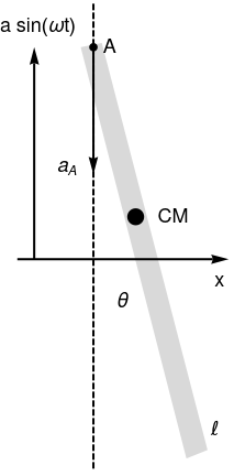
Pendulum with support moving vertically
Let us consider a stiff massless rod of length ℓ and mass m, whose suspension point A oscillates vertically according to yA = 𝑎sin(ωt)
ball = Graphics[{Orange, Disk[{0.27, -0.1}, 0.15]}];
ball2 = Graphics[{Black, Disk[{0.08, 0.6}, 0.02]}];
ball3 = Graphics[{Black, Disk[{-0.02, 1.0}, 0.01]}];
ar = Graphics[{Black, Thickness[0.01], Arrowheads[0.08], Arrow[{{-0.02, 1.0}, {-0.02, 0.7}}]}];
ar2 = Graphics[{Black, Thickness[0.01], Arrowheads[0.08], Arrow[{{-0.2, 0.5}, {0.3, 0.5}}]}];
ar3 = Graphics[{Black, Thickness[0.01], Arrowheads[0.08], Arrow[{{-0.16, 0.5}, {-0.16, 1.0}}]}];
tl = Graphics[{Black, Text[Style["\[ScriptL]", 18, FontFamily -> "Mathematica1"], {0.27, 0.1}]}];
tx = Graphics[{Black, Text[Style["x", 18], {0.28, 0.45}]}];
tcm = Graphics[{Black, Text[Style["CM", 18], {0.17, 0.6}]}];
t2 = Graphics[{Black, Text[Style["\[Theta]", 18], {0.05, 0.4}]}];
line = Graphics[{Black, Dashed, Thick, Line[{{-0.02, 1.1}, {-0.02, 0}}]}];
t3 = Graphics[{Black, Text[Style[Subscript[a, A], 18], {-0.08, 0.72}]}];
t4 = Graphics[{Black, Text[Style["a sin(\[Omega]t)", 18], {-0.15, 1.05}]}];
t5 = Graphics[{Black, Text[Style["A", 18], {0.02, 1.0}]}];
Show[rod, ar, ar2, ar3, tl, tx, ball2, ball3, tcm, t2, t3, line, t4, t5]
|
This equation includes, besides the torque −mgℓ sin(x) of the gravitational force mg, the instantaneous torque of the force of inertial, which depends explicitly on time t.
rec = Graphics[{Pink, Rectangle[{-0.5, -1}, {0.5, 1}]}];
rod = Graphics[{Thickness[0.05], Blue, Line[{{0, 0}, {1, -3}}]}]; line = Graphics[{Dashed, Line[{{0, 0}, {0, -2}}]}]; mass = Graphics[{Gray, Disk[{1, -3}, 0.15]}]; ell = Graphics[{Text[ Style[ToExpression["\ell", TeXForm], FontSize -> 20], {0.7, -1.5}]}]; m = Graphics[Text[Style["m", FontSize -> 20], {1.3, -3}]]; line2 = Graphics[{Dashed, Line[{{0, 0}, {1, 0}}]}]; a = Graphics[{Thickness[0.01], Arrowheads[0.1], Arrow[{{0.8, 0}, {0.8, 1.0}}]}]; txt = Graphics[ Text[Style["A cos(\[Omega]t)", FontSize -> 20], {1.3, 0.6}]]; x = Graphics[Text[Style["x", FontSize -> 20], {0.2, -1.6}]]; Show[rec, rod, m, line, line2, ell, mass, a, txt, x] |
|
| Periodicly excited pivot | Mathematica code |
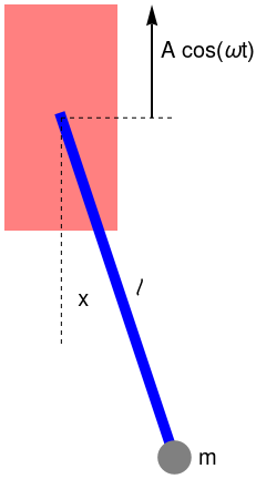
Upon including the frictional torque, which is assumed in this model to be proportional to the momentary value of the angular velocity, with the damping constant γ, we get
rod = Graphics[{Gray, Rectangle[{0.55, 0.65}, {1.05, 0.85}]}];
rod2 = Graphics[{Orange, Rectangle[{-0.4, 2.0}, {1.1, 2.25}]}];
rod3 = Graphics[{Gray, Rectangle[{-0.4, 0.0}, {1.1, -0.1}]}];
rod0 = Graphics[{Blue, Thickness[0.01], Line[{{0.45, 2.0}, {1.5, 0.5}}]}];
ball = Graphics[{Orange, Disk[{1.5, 0.5}, 0.15]}];
damp = Graphics[{Black, Thickness[0.01], Line[{{0.8, 0.0}, {0.8, 0.6}}]}];
damp2 = Graphics[{Black, Thick, Line[{{0.5, 0.9}, {0.5, 0.6}, {1.1, 0.6}, {1.1, 0.9}}]}];
line = Graphics[{Black, Dashed, Thick, Line[{{0.4, 2.1}, {0.4, 2.5}}]}];
line2 = Graphics[{Black, Dashed, Thick, Line[{{0.4, 2.1}, {0.1, 2.5}}]}];
line3 = Graphics[{Black, Dashed, Thick, Line[{{-0.4, -0.05}, {-0.8, -0.05}}]}];
line4 = Graphics[{Black, Dashed, Thick, Line[{{-0.4, 2.1}, {-0.8, 2.1}}]}];
ar = Graphics[{Black, Thickness[0.005], Arrowheads[0.08], Arrow[{{-0.7, -0.05}, {-0.7, 2.1}}]}];
ty = Graphics[{Black, Text[Style["y(t)", 18], {-0.5, 1.0}]}];
tl = Graphics[{Black, Text[Style["\[ScriptL]", 18, FontFamily -> "Mathematica1"], {1.1, 1.3}]}];
t2 = Graphics[{Black, Text[Style["\[Theta]", 18], {0.3, 2.4}]}];
tm1 = Graphics[{Black, Text[Style[Subscript[m, 1], 18], {1.35, 2.1}]}];
tm2 = Graphics[{Black, Text[Style[Subscript[m, 2], 18], {1.5, 0.25}]}];
Show[damp, damp2, damp3, string, ball, rod, rod0, rod2, rod3, line, line2, line3, line4, ar, tl, t2, ty, tm1, tm2]
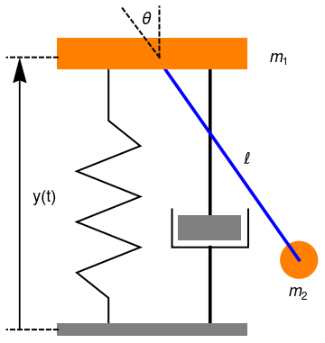
Governing equations are derived using the Lagrange formalism. Considering the frame of reference at the origin placed on the slab and defining in Cartesian coordinates two vectors ry and rθ
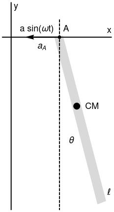
Pendulum with support moving horizontally
Let us consider a pendulumof length ℓ and mass m whose suspension point A oscilates horisontally according to xA = 𝑎 sin ωt. Then its motion is modeled by
ball2 = Graphics[{Black, Disk[{0.08, 0.6}, 0.02]}];
ball3 = Graphics[{Black, Disk[{-0.02, 1.0}, 0.01]}];
ar = Graphics[{Black, Thickness[0.01], Arrowheads[0.08], Arrow[{{-0.02, 1.0}, {-0.22, 1.0}}]}];
tl = Graphics[{Black, Text[Style["\[ScriptL]", 18, FontFamily -> "Mathematica1"], {0.27, 0.1}]}];
tx = Graphics[{Black, Text[Style["x", 18], {0.27, 1.04}]}];
tcm = Graphics[{Black, Text[Style["CM", 18], {0.17, 0.6}]}];
t2 = Graphics[{Black, Text[Style["\[Theta]", 18], {0.05, 0.4}]}];
t3 = Graphics[{Black, Text[Style[Subscript[a, A], 18], {-0.12, 0.95}]}];
t4 = Graphics[{Black, Text[Style["a sin(\[Omega]t)", 18], {-0.15, 1.05}]}]; t5 = Graphics[{Black, Text[Style["A", 18], {0.02, 1.05}]}];
ty = Graphics[{Black, Text[Style["y", 18], {-0.27, 1.18}]}];
line = Graphics[{Black, Dashed, Thick, Line[{{-0.02, 1.1}, {-0.02, 0}}]}];
line2 = Graphics[{Black, Thick, Line[{{-0.35, 1.0}, {0.28, 1.0}}]}];
line3 = Graphics[{Black, Thick, Line[{{-0.3, 0.0}, {-0.3, 1.2}}]}];
Show[rod, ar, tl, tx, ty, ball2, ball3, tcm, t2, t3, line, t4, t5, line2, line3]
The length of the pendulum is increasing by the stretching of the wire due to the weight of the bob. The effective spring constant for a wire of rest length \( \ell_0 \) is
To get a feeling for how rigid and massive the pendulum support must be, we model the support as mass M kept in place by a spring of constant K, as shown in the picture below.
a = Graphics[{Gray, p}]
coil = ParametricPlot[{t + 1.2*Sin[3*t], 1.2*Cos[3*t] - 1.2}, {t, -Pi/6 , 5*Pi - Pi/6}, FrameTicks -> None, PlotStyle -> Black]
line = Graphics[{Thick, Line[{{16.3843645, -1.2}, {20, -1.2}}]}]
r = Graphics[{EdgeForm[{Thick, Blue}], FaceForm[], Rectangle[{20, -5}, {26, 2}]}]
back = RegionPlot[-5 < x < 28 || -7 < y < -5, {x, -5, 28}, {y, -7, -5}, PlotStyle -> LightOrange]
line2 = Graphics[{Thick, Dashed, Line[{{23, -1}, {23, -14}}]}]
line3 = Graphics[{Thick, Line[{{23, -1}, {29, -11.5}}]}]
disk = Graphics[{Pink, Disk[{29.5, -12}, 1]}]
text = Graphics[Text["\[Theta]" , {25.1, -9.5}]]
Show[a, coil, line, r, back, line2, line3, disk, text]
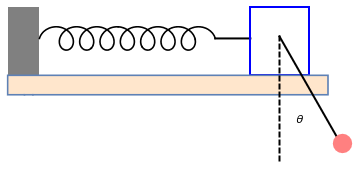
The natural frequency of the support is
Pendulum with moving support
Let us consider a pendulum of length ℓ and mass m whose suspension point A moves with a constant angular frequency ω on a vertical circumference of radius R. In this case, the governing differential equation becomes
ball2 = Graphics[{Black, Disk[{0.105, 0.5}, 0.02]}];
ball3 = Graphics[{Black, Disk[{-0.02, 1.0}, 0.01]}];
ar = Graphics[{Black, Thickness[0.01], Arrowheads[0.08], Arrow[{{-0.02, 1.0}, {-0.138, 0.74}}]}];
line = Graphics[{Black, Dashed, Thick, Line[{{-0.02, 1.1}, {-0.02, 0}}]}];
line2 = Graphics[{Black, Thick, Line[{{-0.2, 0.6}, {0.3, 0.6}}]}];
line3 = Graphics[{Black, Thick, Line[{{-0.2, 0.0}, {-0.2, 1.2}}]}];
line4 = Graphics[{Black, Thick, Line[{{-0.2, 0.6}, {-0.02, 1.0}}]}];
ty = Graphics[{Black, Text[Style["y", 18], {-0.24, 1.18}]}];
tl = Graphics[{Black, Text[Style["\[ScriptL]", 18, FontFamily -> "Mathematica1"], {0.27, 0.1}]}];
tx = Graphics[{Black, Text[Style["x", 18], {0.3, 0.65}]}];
tcm = Graphics[{Black, Text[Style["CM", 18], {0.17, 0.55}]}];
t2 = Graphics[{Black, Text[Style["\[Theta]", 18], {0.05, 0.4}]}];
t3 = Graphics[{Black, Text[Style[Subscript[a, A], 18], {-0.12, 0.95}]}];
t4 = Graphics[{Black, Text[Style["\[Omega]t", 18], {-0.1, 0.65}]}];
t5 = Graphics[{Black, Text[Style["A", 18], {0.02, 1.05}]}];
circle = Graphics[{Blue, Thickness[0.01], Circle[{-0.2, 0.6}, 0.44]}];
Show[circle, rod, ar, tl, tx, ty, ball2, ball3, tcm, t2, t3, t4, t5, line, line2, line3, line4]
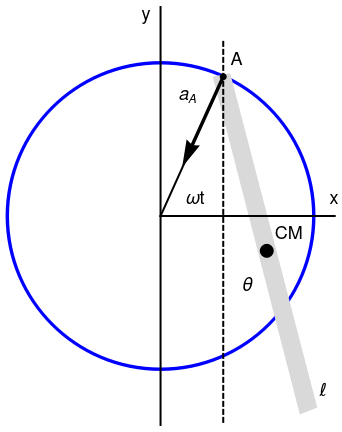
When the pivot is moving on a fixed vertical plane according to xA(t), yA(t), the governing equation reads as
- Kovacic, I., Rand, R., Sah, S.M., Mathieu’s equation and its generalizations: Overview of stability charts and their features, Applied Mechanics Reviews, 2018, Vol. 70, No. 3, 020802-1.
- Rodriguez, L., Torque and the rate of change of angular momentum at an arbitrary point, American Journal of Physics, 2003, Vol. 71, Issue 11, pp. 1201--1203. https://doi.org/10.1119/1.1579498
Return to Mathematica page
Return to the main page (APMA0340)
Return to the Part 1 Matrix Algebra
Return to the Part 2 Linear Systems of Ordinary Differential Equations
Return to the Part 3 Non-linear Systems of Ordinary Differential Equations
Return to the Part 4 Numerical Methods
Return to the Part 5 Fourier Series
Return to the Part 6 Partial Differential Equations
Return to the Part 7 Special Functions