Return to computing page for the first course APMA0330
Return to computing page for the second course APMA0340
Return to Mathematica tutorial for the first course APMA0330
Return to Mathematica tutorial for the second course APMA0340
Return to the main page for the first course APMA0330
Return to the main page for the second course APMA0340
Return to Part II of the course APMA0340
Introduction to Linear Algebra with Mathematica
Glossary
Preface
Systems of differential equations are everywhere. From our relationships and sports games, to complex mathematical problems, differential equations help us analyze the world. They provide concrete models for reality and provide correlations between events, people, and actions. In this Motivation page you will see many of the ways systems of equations impact your life. Whether an engineer or not, systems of differential equations show up everywhere and are crucial to understand in applying your education.
It should be noted that it is often helpful to ground the examples that follow in reality. Read through the examples first and don't focus on the math or equations. Once you have a basic understanding of the problem and solution, and hopefully an appreciation for the elegance of a mathematical model, then look into the method of solution.
Motivation
This section presents motivating examples to study systems of ordinary differential equations (ODE for short),
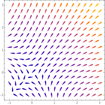
Example 1: Consider the planar system of equations
|
VectorPlot[{y + x^2 , y^2 + x}, {x, -1, 3}, {y, -1, 3},
VectorMarkers -> "Drop"]
|
|
| Direction field for the given system of equations. | Mathematica code |
Each solution x = x(t), y = y(t) of the equation above satisfying the initial condition \[ x(0) > 0 , \qquad y(0) > 0 , \] cannot exist on an interval 0 ≤ t < ∞
In fact, the trajectory of any solution initiating in the first quadrant is contained in the first quadrant. So its global solution does not exist.
Example 2: According to statistical data, about 65% of marriages in the United States end in divorce within a 40-year period, resulting in huge social and economic consequences. The divorce rate for second marriages is even higher, about 75%. Professor John Gottman of the University of Washington identified five types of married couples based on their interactions.
To mathematically model the interplay of a married couple, let x(t) denote a measure of the husband's positivity (e.g., happiness) and let y(t) be the corresponding measurement for the wife's positivity (particular numerical values for such measurements can be found in John's work). In the absence of marital interaction, a single person tends to her/his own ``uninfluenced steady state:'' x0 and y0. This process is modeled by \[ \frac{{\text d}x}{{\text d}t} = h (x-x_0 ) , \qquad \frac{{\text d}y}{{\text d}t} = w (y-y_0 ) . \] After marriage, their interaction can be modeled as \begin{equation} \label{E511.m1} \frac{{\text d}x}{{\text d}t} = h (x-x_0 ) + I_1 (y) , \qquad \frac{{\text d}y}{{\text d}t} = w (y-y_0 ) + I_2 (x), \end{equation} where I1(y) is the influence exerted by the wife on the husband and I2(x) is the influence exerted by the husband on the wife. In a validating style of interaction, these functions can be modeled by \begin{equation} \label{E511.m2} I_k (z) = \begin{cases} a_k z , & \ \mbox{if } z>0 , \\ b_k z , & \ \mbox{if } z<0 \end{cases} \qquad (k=1,2). \end{equation} In a conflict avoiding style of interaction, the spouse who adopts this style avoids interacting with the other spouse through the negative range of his/her emotions. The corresponding function I(z) can be chosen as I(z) = H(z), where H(t) is the Heaviside function. ■
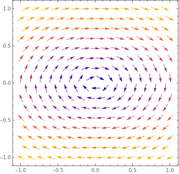
Example 3: To attract your interest in the systems of differential equations, we present a simple model for the dynamics of love affairs (Strogatz 1988). A story written by William Shakespeare about 1594--96, describes a love affair between Romeo and Juliet.
Romeo is in love with Juliet, but in our version of this story, Juliet is a fickle lover. The more Romeo loves her, the more Juliet wants to run away and hide. But when Romeo gets discouraged and backs off, Juliet begins to find him strangely attractive. Romeo, on the other hand, tends to echo her: he warms up when she loves him, and grows cold when she disfavors him.
Let us introduce variables
|
Upon plotting the phase portrait, we see that the governing system has a center at (R, J) = (0,0).
VectorPlot[{2*y, -x}, {x, -1, 1}, {y, -1, 1},
ClippingStyle -> {Blue, Red}]
|
|
| Figure 1: Romeo and Juliet affair. | Mathematica code |
Example 4: Economists and financial analysts often utilize systems of ordinary differential equations (ODE’s) in order to model complex economic phenomena such as resource allocation and optimal growth. These systems often have no explicit analytical solution, but can be visualized and analyzed numerically in order to interpret long-term economic growth in terms of capital accumulation and consumption growth. In 1928, a British philosopher, mathematician, and economist Frank P. Ramsey (1903--1930) discovered what is regarded as the Ramsey growth model, explicating the optimal saving for society using differential equations. The model was expounded upon in 1965 by David Cass (1937--2008) and Tjalling Koopmans (1910--1985), forming the Ramsey--Cass--Koopmans (RCK) model that is currently used widely in macroeconomic theory in order to model optimal growth for an economy possessing labor augmenting technological progress.
We need to remind the main terminology.
- Resource Allocation is the distribution of resources---usually financial---among competing groups of people or programs.
- Optimal Growth: a firm's attempt to balance loss of current utility, as consumption is reduced to finance investment, against the future gain in utility, as the benefit from investment is realized.
- Economic Growth: an increase in the production of economic goods and services, compared from one period of time to another.
- Consumption Growth: an increase in the value of goods and services bought and consumed by people.
- Capital Accumulation: an increase in assets from investments or profits.
- RCK model is the canonical model of optimal growth for an economy with exogenous ‘labor-augmenting’ technological progress.
- Labor Augmenting Technological Progress: technical progress that increases the effective labor input.
- Labor Productivity: the hourly output of a country's economy.
- Labor Supply: the amount of labor workers are willing to offer at various prices.
- Depreciation: the cost of a tangible or physical asset over its useful life or life expectancy.
- Elasticity; a measure of a variable's sensitivity to a change in another variable.
- f(k) = kα is a production function measuring the relative economic output in terms of k and a capital elasticity parameter α (the responsiveness of the output production to changes in the input capital).
- φ is the growth rate of labor productivity (for example, due to technological innovation or efficiency improvements).
- ξ is the growth rate of labor supply (for example, due to migration or population increase).
- δ is the depreciation rate of capital (for example, due to inflation).
- f'(k) = αkα−1 is the rate of change (derivative) of the production function f(k).
- θ is an elasticity parameter indicating the tendency of consumers to smooth out their consumption over time.
- ρ is the rate at which consumers discount their future consumption (for example, by indicating a preference for immediate consumption or attempting to preserve their long-term average consumption).
- Gourinchas, P.-O., The Ramsey-Cass-Koopmans Model, UC Berkeley, 2014.
- Simulating the Ramsey-Cass-Koopmans Model Using MATLAB and Simulink
- The Ramsey-Cass-Koopmans Model
- The Ramsey-Cass-Koopmans Model
- Sargent, Thomas J. & Stachurski, John, Cass-Koopmans Competitive Equilibrium with Python.
Example 5: A neuron or nerve cell is an electrically excitable cell that communicates with other cells via specialized connections called synapses. It is the main component of nervous tissue in all animals except sponges and placozoa. There are only 1011 or so neurons in the human brain, much fewer than the number of non-neural cells such as glia. Yet neurons are unique in the sense that only they can transmit electrical signals over long distances. They allow to understand the neuronal circuits and cortical structure of the brains.
A typical neuron receives inputs from more that 10,000 other neurons through the contacts on its dendritic tree called synapses. The inputs produce electrical transmembrane currents that change the membrane potential of the neuron. Synaptic currents produce changes, called postsynaptic potentials (PSPs for short). Small currents produce small PSPs; large currents produce significant PSPs that can be amplified by the voltage-sensitive channels embedded in the neuronal membrane and lead to the generation of an action potential or spike---an abrupt and transient change of membrane voltage that propagates to other neurons via a long protrusion called an axon.
Such spikes are the main means of communication between neurons. In general, neurons do not fire on their own; they fire as a result of incoming spikes from other neurons. In order to understand how neurons response on incoming inputs, we need to model the dynamics of spike generation mechanisms of neurons.
Neurons can be described as integrators with a threshold: neurons sum incoming PSPs and compare the integrated PSP with a certain voltage value, called the firing threshold. If it is below the threshold, the neuron remains quiescent; when it is above the threshold, the neuron fires an all-or-none spike and resets its membrane potential.
The main observation for modeling neurons is to consider them as a dynamical systems as follows from the Hodgkin--Huxley model. A dynamical system consists of a set of variables that describe its state and a law that defines its evolution with time. The power of the dynamical system approach to neuroscience, as well as to many other sciences, is that we can make conclusions about a system without knowing all details that govern the system evolution.
Let us consider a quiescent neuron whose membrane potential is resting. From the dynamical systems point of view, there are no changes of the state variables of such a neuron: it is in equilibrium position. All the inward currents that depolarize the neuron are balanced, or equilateral, by the outward currents hyperpolarize it. If the neuron remains quiescent despite small disturbances and membrane noise, then we conclude that the equilibrium is stable.
Richard FitzHugh at the National Institute of Health pioneered the phase plane analysis of neuronal models. He introduced in 1961 the simplified model of excitability and showed that one can get the right kind of neuronal dynamics in models lacking conductances and currents. Nagumo et al, (1962) designed a corresponding tunnel diode circuit so the model is called FitzHugh--Nagumo oscillator.
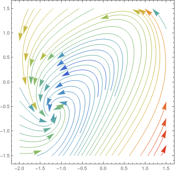
The FitzHugh-Nagumo model (FN-model, for short) is a s follows
- V is the membrane potential,
- W is a recovery variable,
- I is the magnitude of stimulus current.
Actually, the FN-model (5.1) can be generalized to the following one:
|
First, we plot the direction field for homogeneous FitzHugh--Nagumo model when the stimulus parameter is zero:
StreamPlot[{x - x^3 /3 - y, x + 0.7 - 0.8*y}, {x, -2, 1.5}, {y, -1.5,
1.5}, StreamColorFunction -> "Rainbow", StreamPoints -> 42,
StreamScale -> {Full, All, 0.04}]
|
|
| Direction field for the homogeneous FitzHugh--Nagumo model. | Mathematica code |
As it is seen from the direction field, the homogeneous FN-model has a unique equilibrium point (V0, W0). Indeed, solving the system of algebraic equations
You can also repeat the same procedure for Eq.(5.2), but the answer is too complicated to work with. ■
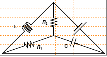
Example 6: We start with two loop circuit:
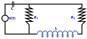
|
coil = ParametricPlot[{1*Cos[t*3 + Pi] + 1.5*t - 9,
2*Sin[t*3] - 8}, {t, 0, 5*Pi}, PlotLabel -> "L", Ticks -> None,
Axes -> False, ImageSize -> Tiny, PlotStyle -> {Thickness[0.01]}];
resistor2 = Graphics[{Thickness[0.01], Line[{{-15, -8}, {-15, -2}, {-17, 0}, {-13, 0}, {-17, 2}, {-13, 2}, {-17, 4}, {-13, 4}, {-17, 6}, {-13, 6}, {-17, 8}, {-13, 8}, {-15, 9}, {-15, 11}}]}, PlotLabel -> Subscript[R, 1], Ticks -> None, Axes -> False]; resistor1 = Graphics[{Thickness[0.01], Line[{{15.5619, -8}, {18, -8}, {18, -2}, {20, 0}, {16, 0}, {20, 2}, {16, 2}, {20, 4}, {16, 4}, {20, 6}, {16, 6}, {20, 8}, {16, 8}, {18, 9}, {18, 11}}]}, PlotLabel -> Subscript[R, 1], Ticks -> None, Axes -> False]; c1 = Graphics[{Thickness[0.01], Circle[{-30, 2}, 2]}]; l1 = Graphics[{Thickness[0.008], Line[{{-25.4, 9.5}, {-25.4, 12.5}}]}]; l2 = Graphics[{Thickness[0.008], Line[{{-24.6, 9.5}, {-24.6, 12.5}}]}]; l3 = Graphics[{Thickness[0.01], Line[{{-10, -8}, {-30, -8}, {-30, 0}}]}]; l4 = Graphics[{Thickness[0.01], Line[{{-30, 4}, {-30, 11}, {-25.4, 11}}]}]; l5 = Graphics[{Thickness[0.01], Line[{{-24.6, 11}, {18, 11}}]}]; txtC = Graphics[ Text[Style["C", Bold, FontSize -> 14, Blue], {-25.5, 8.0}]]; txtV = Graphics[ Text[Style["V(t)", Bold, FontSize -> 14, Blue], {-25.5, 2.0}]]; txtL = Graphics[ Text[Style["L", Bold, FontSize -> 14, Blue], {2.0, -4.5}]]; txtR1 = Graphics[ Text[Style[Subscript[R, 1], Bold, FontSize -> 14, Blue], {-10.5, 2.5}]]; txtR2 = Graphics[ Text[Style[Subscript[R, 2], Bold, FontSize -> 14, Blue], {12.5, 2.5}]]; Show[l1, l2, l3, l4, l5, coil, resistor1, resistor2, c1, txtC, txtV, \ txtL, txtR1, txtR2] |
|
| Two-loop circuit. | Mathematica code |
We denote the current flowing through the left-hand loop by I1 and the current in the right-hand loop by I2 (both in the clockwise direction). The current through the resistor R1 is I1 − I2. The voltage drops on each element are
Now we consider another electric circuit with three loops.
|
connect[pointList_] := {Line[pointList],
Map[Text[Style["", FontSize -> 18]] &,
pointList[[{1, -1}]]]};
resistor[l_ : 1, n_ : 3] := Line[Table[{i l/(4 n), 1/3 Sin[i Pi/2]}, {i, 0, 4 n}]]; gap[l_ : 1] := Line[l {{{0, 0}, {1/3, 0}}, {{2/3, 0}, {1, 0}}}] coil[l_ : 1, n_ : 3] := Module[{scale = l/(5/16 n + 1/2), pts = {{0, 0}, {0, 1}, {1/2, 1}, {1/2, 0}, {1/2, -1}, {5/16, -1}, {5/16, 0}}}, Append[Table[ BezierCurve[scale Map[{d 5/16, 0} + # &, pts]], {d, 0, n - 1}], BezierCurve[scale Map[{5/16 n, 0} + # &, pts[[1 ;; 4]]]]]]; capacitor[l_ : 1] := {gap[l], Line[l {{{1/3, -.5}, {1/3, .5}}, {{2/3, -.5}, {2/3, .5}}}]} battery[l_ : 1] := {gap[ l], {Rectangle[l {1/3, -(2/3)}, l {1/3 + 1/9, 2/3}], Line[l {{2/3, -1}, {2/3, 1}}]}} Options[display] = {Frame -> True, FrameTicks -> None, PlotRange -> All, GridLines -> Automatic, GridLinesStyle -> Directive[Orange, Dashed], AspectRatio -> Automatic}; display[d_, opts : OptionsPattern[]] := Graphics[Style[d, Thick], Join[FilterRules[{opts}, Options[Graphics]], Options[display]]] at[position_, angle_ : 0][obj_] := GeometricTransformation[obj, Composition[TranslationTransform[position], RotationTransform[angle]]] label[s_String, color_ : RGBColor[.3, .5, .8]] := Text@Style[s, FontColor -> color, FontFamily -> "Geneva", FontSize -> Large]; circuit = display[{connect[{{11.5, 0}, {0, 0}, {2.5, 2.5}}], coil[] // at[{2.5, 2.5}, Pi/4], connect[{{3.2, 3.2}, {5.75, 5.75}}], connect[{{5.75, 5.75}, {5.75, 4}}], resistor[] // at[{5.75, 3}, Pi/2], connect[{{5.75, 3}, {5.75, 2}}], connect[{{0, 0}, {2.5, .85}}], capacitor[] // at[{7.5, 1.4}, -Pi/10], connect[{{3.45, 1.2}, {5.75, 2}}], connect[{{5.75, 2}, {7.8, 1.3}}], resistor[] // at[{2.5, .85}, Pi/10], connect[{{8.15, 1.15}, {11.5, 0}}], connect[{{5.75, 5.75}, {8.5, 3}}], battery[] // at[{8.25, 3.25}, -Pi/4], connect[{{8.75, 2.75}, {11.5, 0}}] }] r1 = Graphics[ Text[Style[Subscript[R, 1], Bold, FontSize -> 16, Black], {4.2, 0.7}]]; r2 = Graphics[ Text[Style[Subscript[R, 2], Bold, FontSize -> 16, Black], {4.8, 3.5}]]; txtC = Graphics[ Text[Style["C", Bold, FontSize -> 16, Black], {7.2, 0.8}]]; txtL = Graphics[ Text[Style["L", Bold, FontSize -> 16, Black], {1.5, 3.0}]]; Show[circuit, r1, r2, txtC, txtL] |
|
| Three-loop circuit. | Mathematica code |
We assume that the voltage source satisfies to US standards (Kurtus) with an amplitude of 127 volts and a frequency of 60 Hz to give the frequency-domain function: v(t) = 127 cos(120πt). For the resistors, capacitors, and inductors, I choose to keep the values in simple SI units of ohms, farads, and henries. For each resistor R₁ and R₂, I used a magnitude of 10 ohms. For the capacitor and inductor, I used magnitudes of 5 farads and 5 henries, respectively.
To analyze the AC circuit, I utilized mesh analysis applied to the three loops of the circuit. Using the voltage equations for each of the three types of elements, I derived a system of three equations, but 4 unknowns.
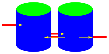
Example 7: This example presents an important application of systems of differential equations to so-called mixed problems. Such a problem usually involves two or more tanks interconnected with pipes. The tanks contain a chemical dissolved in a fluid, which we take as salt (NaCl) and water, respectively. It is often happened that external substance enters one of the tanks and solution leaves the system at some rate. One simplifying assumption that we might make is that the concentration of the substance (salt) is kept uniform in te mixture. Then we can calculate the concentration of the substance in the mixture by dividing the instantaneous amount of salt by the volume of the mixture in the tank at any time t. Multiplying this concentration by the exit rate of the mixture then gives the desired output rate of the substance. At a given time t, we are interested in the amount of salt in each tank.
Two tanks have 200 liters (L) and 300 liters of salt water, respectively. Tank A starts with 10 kg of salt. Tank B starts with 0 kg of salt, so it is full of pure water. 10% salt water enters tank A at 2 L/min. Solution exits the well-mixed tank A at 3 L/min and flows into tank B. Solution exits tank B and enters tank A at 1 L/min. Solution exits tank B and goes into the environment at 2.5 L/min. Therefore, the volume of A is unchanged, and the volume of B changes at a rate of -0.5 L/min.
We assume that the amount of water in the pipe between the tanks is negligible. Let x(t) be the amount of salt in kilograms (kg) in tank A at time t. Let y(t) be the amount of salt in kg in tank B at time t. The concentration in tank A is x/200, and the concentration of salt in tank B is y/(300 −0.5t). The equation describing the rate of change of the amount of salt in tank A is
|
Graphics[{Red, Rectangle[{0, 0.275}, {0.2, 0.3}], Blue,
Rectangle[{0.2, 0}, {0.7, 0.5}], Red,
Rectangle[{0.7, 0.1}, {0.8, 0.125}], Red,
Rectangle[{0.7, 0.15}, {0.8, 0.175}], Blue,
Rectangle[{0.8, 0}, {1.3, 0.5}], Red,
Rectangle[{1.3, 0.1}, {1.5, 0.125}], Green,
Ellipsoid[{0.45, 0.52}, {0.25, 0.1}], Green,
Ellipsoid[{1.05, 0.52}, {0.25, 0.1}], Blue,
Ellipsoid[{1.05, 0}, {0.25, 0.1}], Blue,
Ellipsoid[{0.45, 0}, {0.25, 0.1}], Yellow,
Arrow[{{0, 0.29}, {0.3, 0.29}}], Yellow,
Arrow[{{0.9, 0.11}, {0.6, 0.11}}], Yellow,
Arrow[{{0.7, 0.16}, {0.9, 0.16}}], Yellow,
Arrow[{{1.1, 0.11}, {1.3, 0.11}}]}]
|
|
| Figure 10: Two tanks connected. | Mathematica code |
■
Some Problems from Mechanics
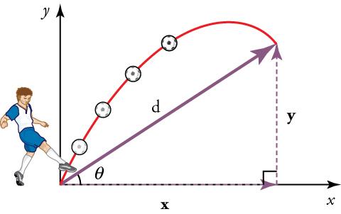
Example 8: A projectile in vacuum is an object upon which the only force acting is gravity, so the influence of air resistance is negligible. More realistic motion under drag force will be considered in the next example. Projectile motion is a form of motion experienced by a launched object. Ballistics (Greek: βάλλειν, romanized: ba'llein, lit. 'to throw') is the science of dynamics that deals with the flight, behavior and effects of projectiles, especially bullets, unguided bombs, rockets, or the like; the science or art of designing and accelerating projectiles so as to achieve a desired performance. In this example, we consider only two dimensional projectile motion in a vacuum. An object dropped from rest is a projectile; an object that is thrown vertically upward is also a projectile. So we first consider a projectile that is thrown upward at an angle α to the horizontal line.
|
|
|
| Vertical trajectories. | Projectile thrown upward at angle α to abscissa. |
Consider an object of mass m which is launched from the origin in a uniform gravitational field g with an initial launch speed of v0 at an angle of α to the horizontal (abscissa). For simplicity, it will be assumed that the motion of the projectile is under the influence of gravity only and that its flight is over level ground so that the end of the flight is at the same level as the beginning. The position vector of the projectile at time t after firing is defined by the vector
|
One can eliminate t from the equations above and get
\begin{equation*}
y(x) = \left( \tan\alpha \right) x - \frac{g\,\sec^2 \alpha}{2\,v_0^2} \, x^2 .
\tag{2.3}
\end{equation*}
The equation above represents a quadratic function: thus, its graph is a parabola.
Therefore, in the absence of air resistance, the path of the projectile is a parabola.
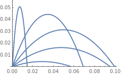
g[x_, a_] = x*(Tan[a]) - (9.81/2)*x^2/Cos[a]^2;
Plot[Table[g[x, c], {c, 0, Pi/2, 0.3}], {x, 0, 0.1}, PlotStyle -> Thick, ImageSize -> 250, PlotRange -> {0, 0.056}] |
|
| Trajectories of a projectile. | Mathematica code |
The time T taken by the projectile to reach the maximum height H, and the range R of the projectile are given by
|
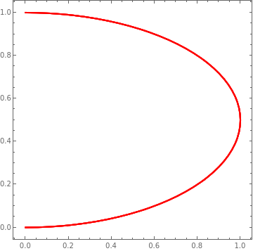
Let (xm, ym) be coordinates of the vertex corresponding to the parabola solution curve, so ym is the maximum height attained and xm is the corresponding horizontal coordinate.
\[
x_m = \frac{v_0^2}{2g} \,\sin \left( 2\alpha \right) , \qquad y_m = \frac{v_0^2}{2g} \,\sin^2 \alpha
\]
ParametricPlot[{Sin[2*a], (Sin[a])^2}, {a, 0, Pi/2}, {r, 0, 1},
Mesh -> Automatic, MeshStyle -> Directive[Thick, Red]]
|
|
| Trajectory of the vertex. | Mathematica code |
|
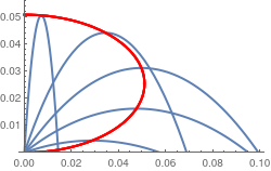
Now we plot trajectories and their corresponding vertices together.
g[x_, a_] = x*(Tan[a]) - (9.81/2)*x^2/Cos[a]^2;
plot = Plot[Table[g[x, c], {c, 0, Pi/2, 0.3}], {x, 0, 0.1}, PlotStyle -> Thick, ImageSize -> 250, PlotRange -> {0, 0.056}]; ver = ParametricPlot[{Sin[2*a]/2/9.81, (Sin[a])^2/2/9.81}, {a, 0, Pi/2}, {r, 0, 1}, Mesh -> Automatic, MeshStyle -> Directive[Thick, Red]]; Show[plot, ver] |
|
| Projectile trajectories along with their vertices. | Mathematica code |
- de Alwise, T., Projectile motion with Mathematica, International Journal of Mathematical Education in Science and Technology, 2000, Vol. 31, No. 5, pp.749--755. doe: 10.1080/002073900434413
- Benacka, I., Stubna, I., Ball launched against an inclined plane---an example of using recurrent sequences in school physics, International Journal of Mathematical Education in Science and Technology, 2009, Vol.40, No. 5, pp. 696--705.
- Bose, S.K., Thoughts on projectile motion, American Journal of Physics, 1985, Vol. 53, No. 2, pp. 175
- de Mestre, N., The Mathematics of Projectiles in Sport, Cambridge University Press, 2012, https://doi.org/10.1017/CBO9780511624032
- Donnelly, D., The parabolic envelope of constant initial speed trajectories, American Journal of Physics, 1992, Vol. 60, No. 12, pp. 1149--1150.
- Fernández-Chapou, J.L., Salas-Brito, A.L. and Vargas, C.A., An elliptic property of parabolic trajectories, American Journal of Physics, 2004, Vol. 72, pp. 1109--1110.
- Hu, H., Yu, J., Another look at Projectile motion, The Physics Teacher, 2000, Vol. 38, No. 10, page 423.
- Padyala, R., An alternative view of the elliptic property of a family of projectile paths, The Physics Teacher, 2019, Vol. 57, No. 9, pp376--377.
- Sarafian, H., On projectile motion, The Physics Teacher, 1999, Vol. 37, No. 2, [[. 86--88.
Example 9: A particular practical interest is a situation when the projectile moves under gravity in a medium whose resistance is not negligible. The drag force acting on the projectile depends on many factors, including material of the projectile, its shape, speed, and some other parameters. Most of these factors are incorporated in the Reynolds number, which we denote by Re to avoid confusion with "Re" (it is a custom to denote as ℜ), which serves to identify a "real part" of a complex number (a standard notation for the Reynolds number is Re). The Reynolds number is the ratio of inertial forces to viscous forces within a fluid that is subjected to relative internal movement due to different fluid velocities. This number was introduced by Sir George Stokes (1819--1903), and popularized by Osborne Reynolds (1842--1912).
Besides gravitational and resistance force, there is another force acting on a ball traveling in air or liquid---the aerodynamic lift due to the backspin of the ball. The air pressure is decreased above the ball and increased below the ball, providing an aerodynamic lift force (Kutta–Joukowski theorem, also Zhukovsky). Therefore, analysis of ball movement in air requires utilization of three forces: gravity, drag, and lift. For a golf ball traveling with speed in range 42 -- 70 m/sec (Reynolds numbers from about 1.25×10⁵ to 1.9×10⁵), the lift force varies approximately linearly with the backspin angular speed.
The air resistance force depends on many things: the speed and direction of motion of the object (called projectile), its shape, size, whether or not it is spinning, the properties of air, whether or not there is any wind, etc.. Any attempt to construct a model of air resistance to be used in projectile motion treating all of these variables rigorously is a tremendously hard job. Since an accurate determination of the resistive force is very complicated, we concentrate our attention on a projectile having shape of a sphere. Fortunately, the dependents of the air resistive force acting on a ball is known and it depends on projectile's speed. For a sphere of radius r moving a fluid of density ρ and viscosity η, the drag force and the Reynolds number are
|
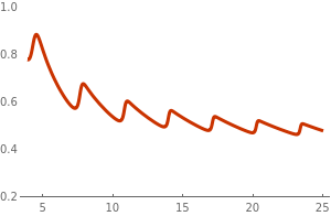
The dependence of the drag force on velocity of a ball moving in air is well documented. Experiments measuring drag force dependence on the ball velocity were conducted by the faculty at MIT, which shows a complicated behavior. For small velocities, it is approximately linear, but then drag force starts closer to the quadratic function with speed increases. At large Reynolds numbers, we observe turbulence behind the ball. So when speed increases (and the Reynolds number exceeds 105), the drag force declines and oscillates as shown in the figure. Such phenomena is observed in baseball (73–75 mm in diameter with a mass of 142 to 149 g) and volleyball (20.7--21.3 cm in diameter with a mass of 260-280 g).
f[t_, y_] = Sin[2.35*t*y]*Cos[t + 1.0*y];
s = NDSolve[{y'[t] == f[t, y[t]], y[0] == 1}, y, {t, 0, 30}]; Plot[Evaluate[y[t] /. s], {t, 3.9, 25}, PlotRange -> {0.2, 1}, PlotTheme -> "Web"] |
|
| Figure 6: Dependence of the drag force on ball's speed. | Mathematica code |
Usually the drag force is modeled by a power function depending on projectile velocity v:
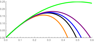
Quadratic Resistance and Speed
Under the conditions of no drift, no wind, an inertial coordinate frame, the density and velocity of sound as functions of the height only, plus the assumption that the only forces with any appreciable effect are gravity and the drag, it is possible to write the equations for a trajectory in the form
|
a=0.3;
s3 = NDSolve[{x''[t] + x'[t]*Sqrt[(x'[t])^2 + (y'[t])^2] == 0, y''[t] + 1 + y'[t]*Sqrt[(x'[t])^2 + (y'[t])^2] == 0, x[0] == 0, x'[0] == Cos[a], y[0] == 0, y'[0] == Sin[a]}, {x[t], y[t]}, {t, 0, 1}]; p3 = ParametricPlot[{x[t], y[t]} /. s3, {t, 0, 0.54}, PlotStyle -> Thickness[0.01], PlotRange -> {{0, 0.55}, {0, 0.33}}]; a=0.5; s5 = NDSolve[{x''[t] + x'[t]*Sqrt[(x'[t])^2 + (y'[t])^2] == 0, y''[t] + 1 + y'[t]*Sqrt[(x'[t])^2 + (y'[t])^2] == 0, x[0] == 0, x'[0] == Cos[a], y[0] == 0, y'[0] == Sin[a]}, {x[t], y[t]}, {t, 0, 1}]; p5 = ParametricPlot[{x[t], y[t]} /. s5, {t, 0, 0.84}, PlotStyle -> {Purple, Thickness[0.01]}, PlotRange -> {{0, 0.55}, {0, 0.33}}]; a=0.7; s7 = NDSolve[{x''[t] + x'[t]*Sqrt[(x'[t])^2 + (y'[t])^2] == 0, y''[t] + 1 + y'[t]*Sqrt[(x'[t])^2 + (y'[t])^2] == 0, x[0] == 0, x'[0] == Cos[a], y[0] == 0, y'[0] == Sin[a]}, {x[t], y[t]}, {t, 0, 2}]; p7 = ParametricPlot[{x[t], y[t]} /. s7, {t, 0, 1.1}, PlotStyle -> {Green, Thickness[0.01]}, PlotRange -> {{0, 0.6}, {0, 0.33}}]]; a=1,0; s10 = NDSolve[{x''[t] + x'[t]*Sqrt[(x'[t])^2 + (y'[t])^2] == 0, y''[t] + 1 + y'[t]*Sqrt[(x'[t])^2 + (y'[t])^2] == 0, x[0] == 0, x'[0] == Cos[a], y[0] == 0, y'[0] == Sin[a]}, {x[t], y[t]}, {t, 0, 2}]; p10 = ParametricPlot[{x[t], y[t]} /. s10, {t, 0, 1.41}, PlotStyle -> {Red, Thickness[0.01]}, PlotRange -> {{0, 0.6}, {0, 0.33}}] a=1,2; s12 = NDSolve[{x''[t] + x'[t]*Sqrt[(x'[t])^2 + (y'[t])^2] == 0, y''[t] + 1 + y'[t]*Sqrt[(x'[t])^2 + (y'[t])^2] == 0, x[0] == 0, x'[0] == Cos[a], y[0] == 0, y'[0] == Sin[a]}, {x[t], y[t]}, {t, 0, 10}]; p12 = ParametricPlot[{x[t], y[t]} /. s12, {t, 0, 1.555}, PlotStyle -> {Black, Thickness[0.01]}, PlotRange -> {{0, 0.6}, {0, 0.33}}]; Show[p12, p10, p7, p5, p3] |
|
| Figure 7: Trajectories of a projectile depending on the initial angle. | Mathematica code |
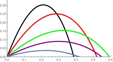
Now we compare all models when a ball is thrown under the same angle, 45°, and the same speed.
|
a = Pi/4;
ss = NDSolve[{x''[t] + x'[t]*(1 + 0.4*Sqrt[(x'[t])^2 + (y'[t])^2]) == 0, y''[t] + 1 + y'[t]*(1 + 0.4*Sqrt[(x'[t])^2 + (y'[t])^2]) == 0, x[0] == 0, x'[0] == Cos[a], y[0] == 0, y'[0] == Sin[a]}, {x[t], y[t]}, {t, 0, 1}]; pp = ParametricPlot[{x[t], y[t]} /. ss, {t, 0, 2.5}, PlotStyle -> {Orange, Thickness[0.01]}, PlotRange -> {{0, 0.6}, {0, 0.25}}]; s = NDSolve[{x''[t] + x'[t] == 0, y''[t] + 1 + y'[t] == 0, x[0] == 0, x'[0] == Cos[a], y[0] == 0, y'[0] == Sin[a]}, {x[t], y[t]}, {t, 0, 1}]; p = ParametricPlot[{x[t], y[t]} /. s, {t, 0, 2.5}, PlotStyle -> {Black, Thickness[0.01]}, PlotRange -> {{0, 0.6}, {0, 0.25}}]; s3 = NDSolve[{x''[t] + Sqrt[(x'[t])^2 + (y'[t])^2]*Abs[x'[t]]^(0.3) == 0, y''[t] + 1 + Sqrt[(x'[t])^2 + (y'[t])^2]*Abs[y'[t]]^(0.3) == 0, x[0] == 0, x'[0] == Cos[a], y[0] == 0, y'[0] == Sin[a]}, {x[t], y[t]}, {t, 0, 1.5}]; p3 = ParametricPlot[{x[t], y[t]} /. s3, {t, 0, 105}, PlotStyle -> {Blue, Thickness[0.01]}, PlotRange -> {{0, 0.6}, {0, 0.25}}]; s2 = NDSolve[{x''[t] + x'[t]*Sqrt[(x'[t])^2 + (y'[t])^2] == 0, y''[t] + 1 + y'[t]*Sqrt[(x'[t])^2 + (y'[t])^2] == 0, x[0] == 0, x'[0] == Cos[a], y[0] == 0, y'[0] == Sin[a]}, {x[t], y[t]}, {t, 0, 1}]; p2 = ParametricPlot[{x[t], y[t]} /. s2, {t, 0, 2.5}, PlotStyle -> {Purple, Thickness[0.01]}, PlotRange -> {{0, 0.6}, {0, 0.25}}]; s0 = NDSolve[{x''[t] == 0, y''[t] + 1 == 0, x[0] == 0, x'[0] == Cos[a], y[0] == 0, y'[0] == Sin[a]}, {x[t], y[t]}, {t, 0, 1}]; p0 = ParametricPlot[{x[t], y[t]} /. s0, {t, 0, 2.5}, PlotStyle -> {Green, Thickness[0.01]}, PlotRange -> {{0, 0.6}, {0, 0.25}}]; Show[pp, p, p3, p2, p0, PlotRange -> {{0, 0.6}, {0, 0.25}}] |
The graphs of trajectories correspond to the following models:
\( \begin{cases} \ddot{x} + \dot{x} \left( 1 + 0.4\,\sqrt{\dot{x}^2 + \dot{y}^2} \right) &=0 , \\ \ddot{y} +1+ + \dot{y} \left( 1 + 0.4\,\sqrt{\dot{x}^2 + \dot{y}^2} \right) &=0 \end{cases} \) (orange),
\( \begin{split} \ddot{x} + \dot{x} =0 , \\ \ddot{y} +1+ + \dot{y} =0 \end{split} \) (black),
\( \begin{cases} \ddot{x} + \sqrt{\dot{x}^2 + \dot{y}^2}\, \dot{x}^{0.3} &=0 , \\ \ddot{y} +1+ + \sqrt{\dot{x}^2 + \dot{y}^2}\, \dot{y}^{0.3} &=0 \end{cases} \) (blue),
\( \begin{cases} \ddot{x} + \dot{x} \,\sqrt{\dot{x}^2 + \dot{y}^2} &=0 , \\ \ddot{y} +1+ + \dot{y} \,\sqrt{\dot{x}^2 + \dot{y}^2} &=0 \end{cases} \) (purple),
and finally, the trajectory of projectile in vacuum (green).
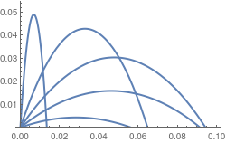
Linear Resistance and Speed
In simple linear resisting medium, the drag force at time t, which acts on the projectile, is taken to be directly proportional to the instantaneous velocity of the projectile at that time and directed in the opposite direction. From Newton’s second law, we have for the horizontal and vertical components of the motion to be
|
Now we plot trajectories in the presence of linear drag force.
gamma = 0.5;
g[x_, a_] = x*(Tan[a] + 9.81/Cos[a]/gamma) + 9.81/gamma^2*Log[1 - gamma*x/Cos[a]]; Plot[Table[g[x, c], {c, 0, Pi/2, 0.3}], {x, 0, 0.1}, PlotStyle -> Thick, ImageSize -> 250, PlotRange -> {0, 0.055}] |
|
| Figure 7: Trajetories in the presence of linear resistance. | Mathematica code |
Considering the value at the maximum, via dy/dx = 0, we obtain
When a projectile is launched vertically upwards (i.e. α = π/2), the horizontal range is xm(π/2) = 0 and its peak heights becomes
The Lambert W function is defined to be the inverse of the function \( w\,e^w = z, \) and is therefore the solution of the defining Lambert equation
The time of flight T is found by setting y = 0 in the formula for y(t), solution of the system of differential equations. Then solving for the time. When this is done, after a little algebraic rearranging of terms
An exact analytic expression for the range R of a projectile in a linear resisting medium can also be found in terms of the Lambert W function.
The angle αmax that maximizes the range of the projectile is found from the angle that satisfies dR/dt = 0. With the availability of an analytical expression for the range as a function of the launch angle α in terms of the Lambert W function, a function whose derivative is known, it is tempting to differentiate one of the equivalent expressions for the range, set the result equal to zero and solve for αmax. This yields
The peak trajectories curve is
- Brancazio, P.J., Trajectory of a fly ball, The Physics Teacher, 1985, Vol. 23, No. 1, pp. 20-23. https://doi.org/10.1119/1.234170
- Coutis, P., Modelling the projectile motion of a cricket ball, International Journal of Mathematical Education in Sciences and Technology, 1998, Vol. 29, No. 6, pp. 789--798.https://doi.org/10.1080/0020739980290601
- Erlichson, H., Maximum projectile range with drag and lift, with particular application to golf, American Journal of Physics, 1983, Vol. 51, No. 4, pp. 357--362. https://doi.org/10.1119/1.13248
- Groetsch, C., Cipra, B., Halley's comment—projectiles with linear resistance, Mathematics Magazine, 1997, Vol. 70, No. 4, pp. 273--280. doi: 10.1080/0025570X.1997.11996553
- Hackborn, W.W., Motion through air: what a drag, Canadian Applied Mathematics Quarterly, 2006, vol. 14, pp. 285–298.
- Hayen, J.C>, Projectile motion in a resistant medium (part I: exact solution and properties), International Journal of Non-Linear Mechanics, 2003, Vol. 38, No. 3, pp.357--369.
- Hernández-Saldaña, H., On the locus formed by the maximum heights of projectile motion with air resistance, European Journal of Physics, 2010, Vol. 31, No. 8, 1319--1329. doi:10.1088/0143-0807/31/6/00
- Kantrowitz, R., The English Galileo and his vision of projectile motion under air resistance, International Journal of Mathematics and Mathematical Sciences, 2020, Article ID 9695053 | https://doi.org/10.1155/2020/9695053
- de Mestre, N., The Mathematics of Projectiles in Sport, Cambridge University Press, 2012, https://doi.org/10.1017/CBO9780511624032
- Mohazzabi, P., When does air resistance become significant in projectile motion? The Physics teacher, 2018, Vol. 68, pp.168--169.
- Packel E and Yuen D 2004 Projectile motion with resistance and the Lambert function, Coll. Math. J., Vol. 35, pp. 337
- Parker, G.W., Projectile motion with air resistance quadratic in the speed, American Journal of Physics, 1977, Vol. 45, No. 7, pp. 606--610.
- Stewart, S.M., An analytic approach to projectile motion in a linear resisting medium, International Journal of Mathematical Education in Science and Technology, 2006, Vol. 37, No. 4, pp. 411-431. doi: 10.1080/00207390600594911
- Warburton, R.D.H. and Wang, J., Analysis of asymptotic motion with air resistance using the Lambert W function, American Journal of Physics, 2004, Vol. 72, pp. 1404--1407.
- Yabushita, K., Yamashita, M., and Tsuboi, K., An analytic solution of projectile motion with the quadratic resistance law using the homotopy analysis method, Journal of Physics A Mathematical and Theoretical 2007, Vol. 40, No 29:8403--8416. doi: 10.1088/1751-8113/40/29/015
Example 10: Consider two pendulums that are coupled by a Hookian spring with spring constant k (see figure below). Suppose that the spring is attached to each rod at a distance 𝑎 from their pivots, and that the pendula (plural from pendulum) are far apart so that the spring can be assumed to be horizontal during their oscillations. Let θ1, θ2 and ℓ1, ℓ2 be the angle of inclination of the shafts with respect to the downward vertical lines and lengths of the rods for the pendula, respectively. The kinetic energy is the sum of kinetic energies of two individual pendula:
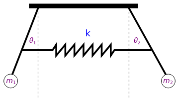
|
polygon = Graphics[Polygon[{{-3, 0}, {3, 0}, {3, 1/4}, {-3, 1/4}}]];
line1 = Graphics[{Dashed, Line[{{2.5, 0}, {2.5, -5}}]}]; line2 = Graphics[{Dashed, Line[{{-2.5, 0}, {-2.5, -5}}]}]; line3 = Graphics[{Thickness[0.01], Line[{{2.5, 0}, {4.5, -3.6}}]}]; line4 = Graphics[{Thickness[0.01], Line[{{-2.5, 0}, {-3.9, -3.6}}]}]; circle1 = Graphics[Circle[{4.66, -4}, 0.38]]; circle2 = Graphics[Circle[{-4.0, -4}, 0.38]]; txt1 = Graphics[ Text[Style[Subscript[m, 1], FontSize -> 14, Purple], {-3.95, -4.0}]]; txt2 = Graphics[ Text[Style[Subscript[m, 2], FontSize -> 14, Purple], {4.68, -4.0}]]; spring = Graphics[{Thickness[0.01], Line[{{-3.35, -2.3}, {-1.7, -2.3}, {-1.5, -2.0}, {-1.5, -2.6}, \ {-1.0, -2.0}, {-1.0, -2.6}, {-0.5, -2}, {-0.5, -2.6}, {0, -2}, {0, \ -2.6}, {0.5, -2.0}, {0.5, -2.6}, {1, -2}, {1, -2.6}, {1.5, -2}, {1.5, \ -2.6}, {1.7, -2.3}, {3.69, -2.3}}]}]; txtk = Graphics[Text[Style["k", FontSize -> 18, Blue], {0.25, -1.4}]]; txt11 = Graphics[ Text[Style[Subscript[\[Theta], 1], FontSize -> 14, Purple], {-2.77, -1.8}]]; txt22 = Graphics[ Text[Style[Subscript[\[Theta], 2], FontSize -> 14, Purple], {2.98, -1.8}]]; Show[polygon, line1, line2, line3, line4, circle1, circle2, txt1, \ txt2, spring, txtk, txt11, txt22] |
|
| Two pendula. | Mathematica code |
Substituting these expressions into the Euler--Lagrange equations \eqref{EqMotiv.2}, we obtain the system of motion:
The case when 𝑎 = ℓ was considered in
Pagliara, M.G., Galimberti, G., et al. Mechanics of two pendulums couples by a stressed spring, American Journal of Physics, 2009, 77, Issue , pp. 834--838. doi: 10.1119/1.3147211
■
Example 11: We consider a problem of a particle moving in straight gravitational tunnel between any two points on the surface of the earth. It is usually hard to trace the origin of ideas, but in our case this problem was known prior to 1898, as it appeas in the work by Edward J. Routh (Cambridge, UK). More information can be found in a note by Philip G. Kirmser (American Journal of Physics, 1966, 34, Issue , p. 701).
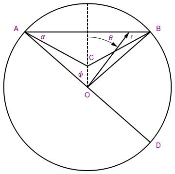
|
circle = Graphics[{Thick, Circle[{0, 0}, 1]}];
diam = Graphics[{Thick, Line[{{-0.75, 0.66}, {0.75, -0.661}}]}]; line = Graphics[{Thick, Line[{{-0.75, 0.66}, {0.75, 0.66}}]}]; line1 = Graphics[{Thick, Line[{{-0.75, 0.66}, {0, 0.25}}]}]; line2 = Graphics[{Thick, Line[{{0.75, 0.661}, {0, 0.25}}]}]; line3 = Graphics[{Thick, Line[{{0.75, 0.66}, {0, 0}}]}]; line4 = Graphics[{Thick, Dashed, Line[{{0, 0}, {0, 1}}]}]; ar = Graphics[{Thick, Arrow[{{0, 0}, {0.5, 0.661}}]}]; arc = Graphics[{Circle[{0, 0}, 0.6, {Pi/2, 0.95}]}]; ar2 = Graphics[{Arrow[{{0.3, 0.52}, {0.36, 0.48}}]}]; txt1 = Graphics[ Text[Style["A", FontSize -> 14, Purple], {-0.85, 0.7}]]; txt2 = Graphics[ Text[Style["B", FontSize -> 14, Purple], {0.85, 0.7}]]; txt3 = Graphics[ Text[Style["C", FontSize -> 14, Purple], {0.05, 0.35}]]; t4 = Graphics[Text[Style["O", FontSize -> 14, Purple], {0., -0.1}]]; t5 = Graphics[Text[Style["D", FontSize -> 14, Purple], {0.85, -0.7}]]; t6 = Graphics[Text[Style["r", FontSize -> 14, Purple], {0.53, 0.6}]]; t7 = Graphics[ Text[Style[\[Alpha], FontSize -> 14, Purple], {-0.53, 0.6}]]; t8 = Graphics[ Text[Style[\[Phi], FontSize -> 14, Purple], {-0.08, 0.15}]]; t9 = Graphics[ Text[Style[\[Theta], FontSize -> 14, Purple], {0.28, 0.59}]]; Show[circle, diam, line, line1, line2, line3, line4, ar, arc, ar2, \ txt1, txt2, txt3, t4, t5, t6, t7, t8, t9] |
|
| Gravitational tunnel. | Mathematica code |
Putting aside various engineering considerations, suppose that a straight hole or tunnel was drilled between any two points on the Earth that is considered as a sphere of radius R ≈ 6,371 kilometres and mass M ≈ 5.972 × 1024 kg. For further simplification, we assume that the Earth is of constant density ρ (which is obviously not true in reality). In order to model such intercontinental frictioness trip, we make a further simplification that the tunell is situated within a plane going though the center of the earth (sphere). This allows us to utilize polar coordinates (r, θ) to identify a position of the particle during such trip. The force of gravity FG acting on a test mass m at radial position r is
Therefore, it would take 42 min to fall through a uniform Earth and the peak velocity at the center would be near 8 km/sec, over 30 times the speed of a typical transatlantic aircraft (about 900 km/hour).
The effect of the daily rotation of the earth (at angular velocity ω) can be taking into account for a path AOD to give
One might want to determine the actual minimal-time path between two points A and B of the surface with no restrictions of linearity imposed. This is more complex than the classical brachistochrone problem in that here the gravitational field is radial instead of rectangular, and is not uniform.
The potential inside the sphere of radius R is \( \Pi = \frac{1}{2}\,mgr^2 /R, \) where m is the mass of the particle and g is the acceleration due to gravity. When the particle starts from rest at the surface, its velocity is obtained from the equation for conservation of energy:
The differential equation for minimum travel time can be written conveniently in a form that expresses the dependence of θ as a function of r (which again follows from the Euler--Lagrange equation for the Lagrangian):
- Cooper, P.W., Through the Earth in Forty Minutes, American Journal of Physics, 1966, 34, Issue 1, p.68. doi: 10.1119/1.1972773
- Cooper, P.W., Further commentary on "Through the Earth in Forty Minutes", American Journal of Physics, 1966, 34, Issue , p.703. doi: 10.1119/1.1973369
- English, L.Q. and Mareno, A., Trajectories of rolling marbles on various tunnels, American Journal of Physics, 2012, 80, Issue 11, pp. 996--1000.
- Klotz, A.R., The gravity tunnel in a non-uniform Eqrth, tunnels, American Journal of Physics, 2015, 83, Issue , p. doi: 10.1119/1.4898780
- Lee, S.M., The isoochronous problem inside the spherically uniform Earth, American Journal of Physics, 1972, 40, Issue , p. 315--317. doi: 10.1119/1.1986515
- Mallett, R.L., Comments on "Through the Earth in Forty Minutes", American Journal of Physics, 1966, 34, Issue , p.231. doi: 10.1119/1.1973208
- Venezian, G., Terrestrial brachistochrone, American Journal of Physics, 1966, 34, Issue , p. 701. doi: 10.1119/1.1973207
Return to Mathematica page
Return to the main page (APMA0340)
Return to the Part 1 Matrix Algebra
Return to the Part 2 Linear Systems of Ordinary Differential Equations
Return to the Part 3 Non-linear Systems of Ordinary Differential Equations
Return to the Part 4 Numerical Methods
Return to the Part 5 Fourier Series
Return to the Part 6 Partial Differential Equations
Return to the Part 7 Special Functions