Preface

---

Sir Isaac Newton (1643--1727) brought to the world the idea of modeling the motion of physical systems with differential equations. However, over the centuries, the most progress in applies in mathematics was made based on developing sophisticated analytical techniques for solving linear systems and their applications. Till the latter portion of the nineteenth century, the normal mathematical techniques are based on an idealized "linearization" of a natural or technological systems that bring the order in our understanding. James Maxwell (1831--1879) was the first who realized that analytical mathematical rules are not always reliable guides to the real world. Carl von Clausewitz (1780--1831), a Prussian general and military theorist, in his book One on War (Chapter 1), emphasized the importance of unpredictability and influence of the initial conditions on outcomes, considering a military action not as a single reaction, but as dynamic interactions between anticipations. Therefore, Clausewitz somehow anticipated today's "chaos theory," but that he perceived and articulated the nature of war as an energy-consuming phenomenon involving competing and interactive factors:

Although our intellect always longs for clarity and certainty, our nature often finds uncertainty fascinating.

Around 1975, after three centuries of study, scientists in large numbers around the world suddenly became aware that there is a special kind of motion that is now now called “chaos”. Chaos is the mathematical theory of dynamical systems that are highly sensitive to initial conditions – a response popularly referred to as the “butterfly effect”. Small differences in initial conditions (such as those due to rounding errors in numerical computation or measurement uncertainty) yield widely diverging outcomes for such dynamical systems, rendering long-term prediction impossible in general. This happens even though these systems are deterministic, meaning that their future behavior is fully determined by their initial conditions,with no random (stochastic) elements involved. The new motion is erratic, but not simply quasiperiodic with a large number of periods, not a kind of equilibrium solution, and not necessarily due to a large number of interacting particles. By the 1960s, there were small groups of mathematicians, particularly in Berkeley (USA), Cambridge (MIT, USA), and in Moscow (Russia), striving to understand this kind of motion that we now call chaos. But only with the advent of personal computers, with screens capable of displaying graphics, have scientists and engineers been able to see that important equations in their own specialties had such solutions, at least for some ranges of parameters that appear in the equations.

Over decades, chaos has been observed in nature (weather and climate, dynamics of satellites in the solar system, time evolution of the magnetic field of celestial bodies, and population growth in ecology) and laboratory (electrical circuits, lasers, chemical reactions, fluid dynamics, mechanical systems, and magneto-mechanical devices). Chaotic behavior has also found numerous applications in electrical and engineering, information and communication technologies, biology and medicine. By now, many chaotic models have been developed and studied in great detail, but they continue to present surprises and raise questions. Recently, the subject of chaos and nonlinear dynamics has received a tremendous amount of attention. However, due to its inherent complexity and intensively numerical nature, it is hard to give a relatively elementary treatment.

When the number of dependent variables in the dynamic system exceeds two, the classification of equilibria points presented in planar case previously is not sufficient. One problem is that there is simply a greater number of possible cases that can occur, and the number increases with the order of the system (and the dimension of the phase space). Another issue is the difficulty of graphing trajectories accurately in a phase space of higher than two dimensions; even in three dimensions, it may not be easy to construct a clear and understandable plot of the trajectories, and it becomes more difficult as the number of variables increases. Finally, there are different and very complex phenomena that can occur, and do frequently occur, in systems of third and higher order that are not present in second order systems.

All considered systems of differential equations are deterministic because they contain no random, noisy, or stochastic terms. All their solutions are unique and determine a unique flow which is valid for all time. However, some solution graphs and phase plots for system of ordinary differential equations are so irregular that they display very little apparent order and provide no prediction in solution behavior. Therefore, it is a custom to call such systems chaotic. These systems of equations) are not stiff or otherwise difficult to integrate numerically---their chaotic nature does not depend on numerical solvers in use.

Inability of numerical approximations to predict the actual time evolution of a solution stimulates theoretical qualitative analysis of such systems. Non-linear systems of ordinary differential equations (ODEs) are not well understood. Utilizing numerical experiments may be not adequate because they are based only on a finite number of numerical experiments at a finite number of parameter values, each with only finite accuracy. It is always possible that, for some parameter values we have not examined, the behavior is completely different, or that there are strange things going on in some region of phase space that we have not investigated. Such possibilities should be never dismissed. Therefore, numerical experiments should be supplemented with theoretical investigations.

Although chaos is a well-established phenomenon, its strict mathematical definition is still under scrutiny. There are several techniques to find whether any system is chaotic or not. We mention three of them, but only the first one will be used in this tutorial, with ocation demonstrations of the second one.

• Dense filled phase portraits
• Poincaré map or section
• Lyapunov exponents

Examples of Chaotic Equations

---

Chaotic systems are dynamical systems that appear to be random and disorderly but are actually governed by underlying patterns. These systems are highly influenced by initial conditions since a slight change in initial values can cause a very different outcome, a property which is popularly known as the butterfly effect. We now know a great number of sets of ordinary differential equations derived from an even greater number of real world problems, which have chaotic looking solutions, in some respect or other. The list of chaotic systems can be found on the web.

The Rabinovich–Fabrikant system is a set of equations developed by Russian (of Jewish descent) scientists Mikhail Rabinovich and Anatoly Fabrikant in 1979 to model waves in non-equilibrium media. Traditional nonlinear dynamics with relation to physical applications (mainly electronics and radio) was developed by Mandelshtam, Andronov, etc. in around 1930 and it was based on so-called "qualitative theory of differential equations." They gave full and complete analyses of two-dimensional systems and showed that the only attractors in 2D systems were equilibrium states and limit cycles. The higher dimensional systems were mainly "terra incognita" till "strange attractors" were discovered in 3D systems, starting from Lorenz system, which was supposed to describe weather dynamics. It has become clear then, that 3D systems (and weather therefore) may exhibit chaotic behavior, which can't be fully predictable.

Rabinovich and Fabrikant were the first who discovered the practical chaotic system, describing real physical effect (modulational instability), which can be found in multiple physical applications. Unlike to Lorents system that served to mathematically demonstrate chaotic behavior of solutions to 3D systems, the RF model was driven by practical applications. As for possible application of RF strange attractor, imagine, for example, waves in some medium with dispersion (plasma or fluid or any other), where waves exited with a certain frequency. Because of dispersion, they cannot generate harmonics or subharmonics. Instead, when they propagate, they exhibit modulational instability, generating satellite harmonics, which are beyond the excitation range and therefore are subject to dissipation. This may happen, for example, in a resonator, where frequencies are discrete. A classical rubi laser could be a good example of this. That is when a strange attractor may appear given certain parameters.

 

		This system is given by a set of three coupled ordinary differential equations as \begin{equation} \label{EqChaos.1} \begin{split} \dot{x} &= y \left( z-1 + x^2 \right) + \gamma \,x , \\ \dot{y} &= x \left( 3z + 1 - x^2 \right) + \gamma \, y , \\ \dot{z} &= -2z \left( \alpha + xy \right) , \end{split} \end{equation} where α and γ are constants that control the evolution of the system. For some values of α and γ, the system is chaotic, but for others it is periodic. Bifurcation studies have shown that for α = 1.2, γ = 0.87 we have a chaotic system and α = 1.5, γ = 0.55 correspond to a non-chaotic system.
Mikhail Rabinovich				Anatoly Fabrikant

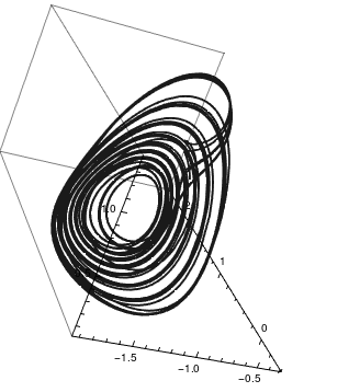
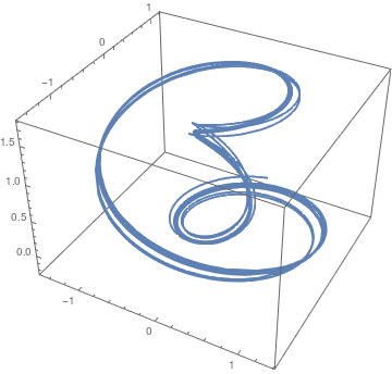
		We plot solutions to RF system when α = 1.1 and γ = 0.87 with the initial conditions \[ x(0) = -1, \quad y(0) = 0, \quad z(0) = 0.5. \] a = 1.1; gamma = 0.87; sol = NDSolve[{x'[t] == y[t]*(z[t] - 1 + (x[t])^2) + gamma*x[t], y'[t] == x[t]*(3*z[t] + 1 - (x[t])^2) + gamma*y[t], z'[t] == -2*z[t]*(a + x[t]*y[t]), x[0] == -1, y[0] == 0, z[0] == 0.5}, {x, y, z}, {t, 0, 100}] ParametricPlot3D[Evaluate[{x[t], y[t], z[t]} /. sol], {t, 0, 100}, PlotRange -> All, PlotTheme -> "Monochrome"]
Rabinovich–Fabrikant system		Mathematica code

Historical notes about Rabinovich–Fabrikant system References for the Rabinovich–Fabrikant systems

The Genesio equation is

where 𝑎, b, and c are some constants. Numerical experiments show that system \eqref{EqChaos.2} exhibits a chaotic behavior when

		a = 1.2; b = 2.92; c = 6; sol = NDSolve[{x'[t] == y[t], y'[t] == z[t], z'[t] + a*z[t] + b*y[t] + c*x[t] - (x[t])^2 == 0, x[0] == 0.2, y[0] == -0.3, z[0] == 1}, {x, y, z}, {t, 0, 200}]; ParametricPlot3D[Evaluate[{x[t], y[t], z[t]} /. sol], {t, 0, 200}, PlotRange -> All, PlotTheme -> "Monochrome"]
Genesio equation		Mathematica code

 

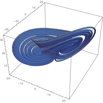
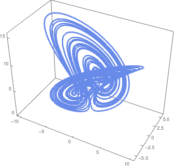
The Chen double scroll attractor is a system of ODEs is models morphogenesis in higher organisms. with \[ a = 40, \quad b =3, \quad c = 28 \qquad\mbox{and initial conditions} \qquad x_0 = -0.1, \quad y_0 = 0.5, \quad z_0 = -0.6 . \]

		(* Set the parameters *) a = 40; b = 3; c = 28; (* Set the differential equation *) F1[x_, y_, z_] := a (y - x) F2[x_, y_, z_] := (c - a) x - x z + c y F3[x_, y_, z_] := x y - b z (* Set the initial conditions *) x0 = -0.1; y0 = 0.5; z0 = -0.6; ta = 2; (* Solve, keeping the final value because we are removing transient behavior and waiting for the solution to converge to the attractor *) ap = NDSolve[{xa'[t] == F1[xa[t], ya[t], za[t]], ya'[t] == F2[xa[t], ya[t], za[t]], za'[t] == F3[xa[t], ya[t], za[t]], xa[0] == x0, ya[0] == y0, za[0] == z0}, {xa, ya, za}, {t, 0, ta},MaxSteps -> Infinity] (* Start a new computation at the place where the last solution ended. *) x1 = xa[ta] /. ap; y1 = ya[ta] /. ap; z1 = za[ta] /. ap; tb = 50; (* Solve again, except this time starting at the place the solution ended the last time *) bp = NDSolve[{xb'[t] == F1[xb[t], yb[t], zb[t]], yb'[t] == F2[xb[t], yb[t], zb[t]], zb'[t] == F3[xb[t], yb[t], zb[t]],xb[0]==x1, yb[0]==y1, zb[0]==z1},{xb, yb, zb}, {t, 0, tb}, MaxSteps -> Infinity] (* Plot the attractor for viewing on screen *) ParametricPlot3D[{xb[t], yb[t], zb[t]} /. bp,{t, 0, tb}, PlotRange -> All] (* Plot again in 3D *) cp = ParametricPlot3D[{xb[t], yb[t], zb[t]} /. bp,{t, 0, tb}, PlotStyle -> Tube[.5], PlotPoints -> 100, PlotRange -> All]
Chen double scroll.		Mathematica code

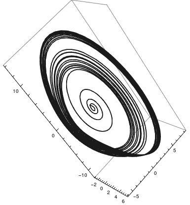
The Langford attractor appear in three dimensional (3D) systems of ODEs.

		We use the following numerical values \[ a=0.95, \quad b = 0.7, \quad c = 0.6, \quad d=3.5, \quad e= 0.25, \] and initial conditions: \[ x_0 = 0.1, \quad y_0 =1, \quad z_0 = 0. \] F1[x_, y_, z_] := x (z - 0.7) - 3.5*y; F2[x_, y_, z_] := 3.5*x + (z - 0.7)*y; F3[x_, y_, z_] := 0.6 + 0.95*z - z^3 /3 - (x^2 + y^2)*(1 + 0.25*z) + 0.1*z*x^3; ap = NDSolve[{xa'[t] == F1[xa[t], ya[t], za[t]], ya'[t] == F2[xa[t], ya[t], za[t]], za'[t] == F3[xa[t], ya[t], za[t]], xa[0] == x0, ya[0] == y0, za[0] == z0}, {x, y, z}, {t, 0, 50}, MaxSteps -> Infinity] ParametricPlot3D[Evaluate[{x[t], y[t], z[t]} /. ap], {t, 0, 50}, PlotRange -> All]
Langford attractor.		Mathematica code

The Rucklidge attractor appear in three dimensional (3D) systems of ODEs.

		We use the following numerical values \[ \kappa = -2, \quad \lambda = -6.7 \] and initial conditions: \[ x_0 = 1, \quad y_0 = 0, \quad z_0 = 4.5 . \] solution = NDSolve[{x'[t] == -2*x[t] + 6.7*y[t] - y[t]*z[t], y'[t] == x[t], z'[t] == -z[t] + (y[t])^2, x[0] == 1, y[0] == 0, z[0] == 4.5}, {x, y, z}, {t, 0, 150}] ParametricPlot3D[Evaluate[{x[t], y[t], z[t]} /. ap], {t, 0, 150}, PlotRange -> All < PlotTheme -> "Business"]
Rucklidge attractor.		Mathematica code

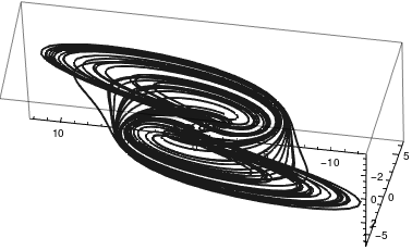
The Arneodo attractor is

where 𝑎, b, and c are some constants. Numerical experiments show that system \eqref{EqChaos.8} exhibits a chaotic behavior when

		a = -5.5; b = 3.5; c = 1; sol = NDSolve[{x'[t] == y[t], y'[t] == z[t], z'[t] + a*x[t] + b*y[t] + z[t] + (x[t])^3 == 0, x[0] == 0.2, y[0] == 0.2, z[0] == -0.75}, {x, y, z}, {t, 0, 200}]; ParametricPlot3D[Evaluate[{x[t], y[t], z[t]} /. sol], {t, 0, 200}, PlotRange -> All, PlotTheme -> "Monochrome"]
Arneodo attractor		Mathematica code

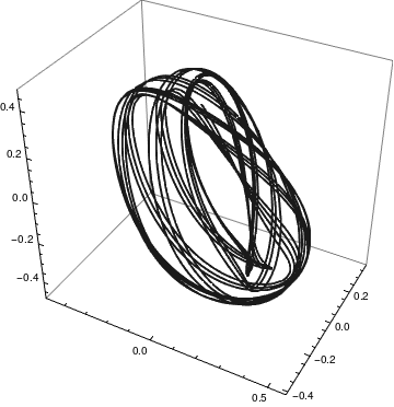
The Hénon-Heiles invariant torus models the motion of individual stars as affected by the rest of a galaxy. Unlike the other models, this is a four-dimensional example. We project and only plot(𝑥,𝑦,𝑧). The system is Hamiltonian, so the chaotic solutions are not strange attractor.

Initial conditions:

		solution = NDSolve[{x'[t] == z[t], y'[t] == w[t], z'[t] == -x[t] - 2*x[t]*y[t], w'[t] == -y[t] - (x[t])^2 + (y[t])^2, x[0] == 0, y[0] == 0, z[0] == 0.35, w[0] == -0.3}, {x, y, z, w}, {t, 0, 200}] ParametricPlot3D[ Evaluate[{x[t], y[t], z[t]} /. solution], {t, 0, 150}, PlotRange -> All, PlotTheme -> "Monochrome"]
Hénon-Heiles invariant torus.		Mathematica code

Poincaré Map

---

A dynamical system is any system that allows one to determine (at least theoretically) the future states of the system provided the present value. In this tutorial, we consider dynamical systems that are generated by differential equations.

In dynamical systems, a first recurrence map or Poincaré map, named after Henri Poincaré (1854--1912), is the intersection of a periodic orbit in the state space of a continuous dynamical system with a certain lower-dimensional subspace, called the Poincaré section, transversal to the flow of the system or stroboscopic section. More precisely, one considers a periodic orbit with initial conditions within a section of the space, which leaves that section afterwards, and observes the point at which this orbit first returns to the section. One then creates a map to send the first point to the second, hence the name first recurrence map. The transversality of the Poincaré section means that periodic orbits starting on the subspace flow through it and not parallel to it.

A Poincaré map can be interpreted as a discrete dynamical system with a state space that is one dimension smaller than the original continuous dynamical system. Because it preserves many properties of periodic and quasiperiodic orbits of the original system and has a lower-dimensional state space, it is often used for analyzing the original system in a simpler way. In practice this is not always possible as there is no general method to construct a Poincaré map.

Example 1: Forced harmonic oscillator Example 2: Forced damped harmonic oscillator Example 3: Mathieu equation

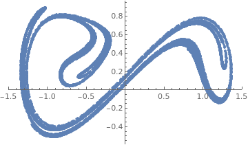
		Consider the Duffing equation subject to the homogeneous initial conditions: \[ \ddot{x}(t) + a\,\dot{x}(t) -x(t) + x^3 (t) = b\,\cos t, \qquad x(0) =0 , \quad \dot{x} (0) = 0. \] data = Block[{a = 0.21, b = 0.31}, Reap[NDSolve[{x''[t] + a*x'[t] - x[t] + x[t]^3 == b*Cos[t], x[0] == 0, x'[0] == 0, WhenEvent[Mod[t, 2*Pi] == 0, Sow[{x[t], x'[t]}]]}, {}, {t, 0, 100000}, MaxSteps -> Infinity]]][[-1, 1]]; ListPlot[data, PlotRange->{{-1.5,1.5},All}, PlotStyle->PointSize[0.01]]
Poincaré section for the Duffing equation.		Mathematica code

 

References

 

Return to Mathematica page
Return to the main page (APMA0340)
Return to the Part 1 Matrix Algebra
Return to the Part 2 Linear Systems of Ordinary Differential Equations
Return to the Part 3 Non-linear Systems of Ordinary Differential Equations
Return to the Part 4 Numerical Methods
Return to the Part 5 Fourier Series
Return to the Part 6 Partial Differential Equations
Return to the Part 7 Special Functions

 

Complex dynamics and chaos in commutable pendulum. Revista Mexicana de Fisica 58(1):6-12 · February 2012 Valeri Nosov, H Dominguez, J.A. Ortega-Herrera, Jesus Alberto Meda Campaña Yet Another Chaotic Attractor  International Journal of Bifurcation and Chaos 9(07):1465-1466 · July 1999 doi: 10.1142/S0218127499001024 Guanrong Chen, Tetsushi Ueta Simplest Chaotic System with a Hyperbolic Sine and Its Applications in DCSK Scheme  IET Communications 12(7) · January 2018 with 165 doi: 10.1049/iet-com.2017.0455 izhao Liu, Julien Clinton Sprott, haonan Wang, Yide Ma