Preface

This section concerns about numerical solutions to the Laplace equation.

Return to computing page for the first course APMA0330
Return to computing page for the second course APMA0340
Return to Mathematica tutorial for the first course APMA0330
Return to Mathematica tutorial for the second course APMA0340
Return to the main page for the first course APMA0330
Return to the main page for the second course APMA0340
Return to Part VI of the course APMA0340
Introduction to Linear Algebra with Mathematica

Glossary

Numerical Solutions to Laplace Equations

In this section, we discuss some algorithms to solve numerically boundary value porblems for Laplace's equation (∇²u = 0), Poisson's equation (∇²u = g(x,y)), and Helmholtz's equation (∇²u + k(x,y) u = g(x,y)). We start with the Dirichlet problem in a rectangle \( R = [0,a] \times [0,b] . \)

The Laplacian operator must be expressed in a discrete form suitable for numerical computations. The formula for approximating \( f'' (x) \) is obtained from

\[ f'' (x) = \frac{f(x+h) -2\,f(x) + f(x-h)}{h^2} +O(h^2 ) . \]

When this formula is applied to the Laplace equation involving approximation of partial derivatives u_xx and u_yy and the results are added, we obtain

\[ \Delta u = \frac{1}{h^2} \left[ u(x+h,y) + u(x-h,y) + u(x,y+h) + u(x,y-h) -4\,u(x,y) \right] +O(h^2 ) . \]

Suppose that we seek a solution of the Laplace equation in the rectangular domain [0,a]×[0,b]. Assume that the rectangle is divided into (n-1)×(m-1) squares with side h so that a = nh and b = mh because we assume also that b/a = m/n.

l0 = Graphics[{Thick,Line[{{0,0},{8,0}}]}];
l1 = Graphics[{Thick,Line[{{0,1},{8,1}}]}];
l2 = Graphics[{Thick,Line[{{0,2},{8,2}}]}];
l3 = Graphics[{Thick,Line[{{0,3},{8,3}}]}];
l4 = Graphics[{Thick,Line[{{0,4},{8,4}}]}];
l5 = Graphics[{Thick,Line[{{0,5},{8,5}}]}];
la0 = Graphics[{Thick,Line[{{0,0},{0,5}}]}];
la1 = Graphics[{Thick,Line[{{1,0},{1,5}}]}];
la2 = Graphics[{Thick,Line[{{2,0},{2,5}}]}];
la3 = Graphics[{Thick,Line[{{3,0},{3,5}}]}];
la4 = Graphics[{Thick,Line[{{4,0},{4,5}}]}];
la5 = Graphics[{Thick,Line[{{5,0},{5,5}}]}];
la6 = Graphics[{Thick,Line[{{6,0},{6,5}}]}];
la7 = Graphics[{Thick,Line[{{7,0},{7,5}}]}];
la8 = Graphics[{Thick,Line[{{8,0},{8,5}}]}];
d0 = Graphics[{Orange, Disk[{4, 3}, 0.15]}];
d1 = Graphics[{Orange, Disk[{4, 4}, 0.15]}];
d2 = Graphics[{Orange, Disk[{4, 2}, 0.15]}];
d3 = Graphics[{Orange, Disk[{3, 3}, 0.15]}];
d4 = Graphics[{Orange, Disk[{5, 3}, 0.15]}];
r1 = Graphics[ Text[Style["\!\(\*SubscriptBox[\(x\), \(i\)]\)", Medium], {4, -0.3}]];
r2 = Graphics[ Text[Style["\!\(\*SubscriptBox[\(x\), \(i-1\)]\)", Medium], {3, -0.3}]];
r3 = Graphics[ Text[Style["\!\(\*SubscriptBox[\(x\), \(i+1\)]\)", Medium], {5, -0.3}]];
r4 = Graphics[ Text[Style["\!\(\*SubscriptBox[\(x\), \(n-1\)]\)", Medium], {7, -0.3}]];
r5 = Graphics[ Text[Style["\!\(\*SubscriptBox[\(x\), \(n\)]\)", Medium], {8, -0.3}]];
r6 = Graphics[ Text[Style["\!\(\*SubscriptBox[\(x\), \(2\)]\)", Medium], {1, -0.3}]];
r7 = Graphics[ Text[Style["\!\(\*SubscriptBox[\(x\), \(1\)]\)", Medium], {0, -0.3}]];
t0 = Graphics[ Text[Style["\!\(\*SubscriptBox[\(y\), \(1\)]\)", Medium], {-0.3, 0}]];
t1 = Graphics[ Text[Style["\!\(\*SubscriptBox[\(y\), \(j-1\)]\)", Medium], {-0.4, 2}]];
t2 = Graphics[ Text[Style["\!\(\*SubscriptBox[\(y\), \(j\)]\)", Medium], {-0.3, 3}]];
t3 = Graphics[ Text[Style["\!\(\*SubscriptBox[\(y\), \(j+1\)]\)", Medium], {-0.4, 4}]];
t4 = Graphics[ Text[Style["\!\(\*SubscriptBox[\(y\), \(m\)]\)", Medium], {-0.3, 5}]];
Show[l0,l1,l2,l3,l4,l5,la0,la1,la2,la3,la4,la5,la6,la7,la8,d0, d1, d2, d3, d4, r1,r2,r3,r4,r5,r6,r7, t0,t1,t2,t3,t4]

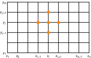
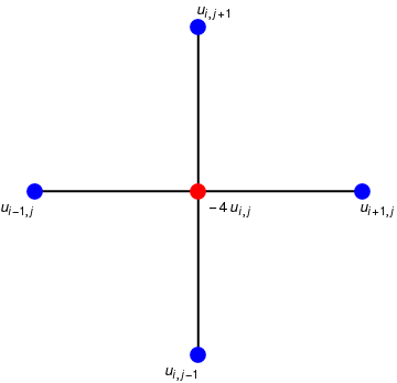
The grid used with Laplace's difference equation

To solve Laplace's equation, we impose the approximation

\[ \frac{1}{h^2} \left[ u(x+h,y) + u(x-h,y) + u(x,y+h) + u(x,y-h) -4\,u(x,y) \right] =0, \]

which has order of accuracy O(h²) at all interior grid points \( (x,y) = (x_i , y_j ) \) for i = 2, 3, …, n-1 and j = 2, 3, …, m-1. The grid points are uniformly spaced: \( x_{i+1} = x_i + h, \ x_{i-1} = x_i -h, \ y_{j+1} = y_j +h , \ y_{j-1} = y_j -h . \) Using notation u_i,j for \( u (x_i , y_j ) , \) the discrete Laplace equation can be written as

\[ \Delta u_{i,j} \approx \frac{u_{i+1,j} + u_{i-1,j} + u_{i,j+1} + u_{i,j-1} - 4\,u_{i,j}}{h^2} =0 , \]

which is known as the five-point difference formula for Laplace's equation. This formula is usually called the five-point stencil of a point in the grid is a stencil made up of the point itself together with its four "neighbors". It is used to write finite difference approximations to derivatives at grid points. This formula relates the function value \( u_{i+1,j} \equiv u(x_{i+1}, y_j ) \) to its four neighboring values u_i+1,j, u_i-1,j, u_i,j+1, and u_i,j-1, as shown in stencil below. The multiple h² can be eliminated and we obtain the Laplacian computational formula:

\[ u_{i+1,j} + u_{i-1,j} + u_{i,j+1} + u_{i,j-1} - 4\,u_{i,j} =0 . \]

l1 = Graphics[{Thick,Line[{{-2,0},{2,0}}]}];
l2 = Graphics[{Thick,Line[{{0,-2},{0,2}}]}];
d0 = Graphics[{Red, Disk[{0, 0}, 0.1]}];
d1 = Graphics[{Blue, Disk[{0, 2}, 0.1]}];
d2 = Graphics[{Blue, Disk[{0, -2}, 0.1]}];
d3 = Graphics[{Blue, Disk[{2, 0}, 0.1]}];
d4 = Graphics[{Blue, Disk[{-2, 0}, 0.1]}];
t0 = Graphics[ Text[Style["\!\(\*SubscriptBox[\(-4 u\), \(i,j\)]\)", Medium], {0.4, -0.2}]];
t1 = Graphics[ Text[Style["\!\(\*SubscriptBox[\(u\), \(i-1,j\)]\)", Medium], {-2.2, -0.2}]];
t2 = Graphics[ Text[Style["\!\(\*SubscriptBox[\(u\), \(i+1,j\)]\)", Medium], {2.2, -0.2}]];
t3 = Graphics[ Text[Style["\!\(\*SubscriptBox[\(u\), \(i,j+1\)]\)", Medium], {0.2, 2.2}]];
t4 = Graphics[ Text[Style["\!\(\*SubscriptBox[\(u\), \(i,j-1\)]\)", Medium], {-0.2, -2.2}]];
Show[l1,l2,d0,d1,d2,d3,d4, t0,t1,t2,t3,t4]

Assume that the values u(x,y) are known at the following boundary grid points:

\begin{align*} u(x_1,y_j ) &= u_{1,j} \qquad&\mbox{for } 2 \le j \le m-1 \qquad &(\mbox{on the left}), \\ u(x_i, y_1 ) &= u_{i,1} \qquad&\mbox{for } 2 \le i \le n-1 \qquad &(\mbox{on the bottom}), \\ u(x_n,y_j ) &= u_{1,j} \qquad&\mbox{for } 2 \le j \le m-1 \qquad &(\mbox{on the right}), \\ u(x_i, y_m ) &= u_{i,1} \qquad&\mbox{for } 2 \le i \le n-1 \qquad &(\mbox{on the top}) . \end{align*}

Then applying the Laplace computational formula at each of the interior points of R will creat a linear system of (n-2) equations in (n-2) unknowns, which is solved to obtain approximations to u(x,y) at the interior points of R.

Program (Dirichlet method for Laplace's equation): to approximate the solution of \( u_{xx} + u_{yy} =0 \) over \( R = \{\,(x,y) \,:\, 0 \le x \le a , \ 0 \le y \le b \) with \( u(x,0) = f_0 (x), \ u(x,b) = f_b (x) , \) for 0 ≤ x ≤ a;, and \( u(0,y) = g_0 (y), \ u(a,y) = g_a (y) , \) for 0 ≤ y ≤ b. It is assumed that Δx = Δy = h and that integers n and m exist so that a=nh and b=mh.


function U=dirichlet(f0,fb,g0,ga,a,b,h,tol,max1)
% Input  -- f0,fb,g0,ga are boundary functions input as a strings
%        -- a and b right end points of [0,a] and [0,b]
%        -- h step size
%        -- tol is the tolerance
%        -- max1 
% Output -- U solution matrix; 
% Initialize parameters and U 
n=fix(a/h)+1;
m=fix(b/h)+1; 
ave=(a*(feval(f0,0)+feval(fb,0))+b*(feval(g0,0)+feval(ga,0)))/(2*a+2*b);
U=ave*ones(n,m);
% Boundary conditions 
U(1,1:m)=feval(g0,0:h:(m-1)*h))';
U(n,1:m)=feval(ga,0:h:(m-1)*h))';
U(1:n,1)=feval(fa,0:h:(n-1)*h))';
U(1:n,m)=feval(fb,0:h:(n-1)*h))';
U(1,1)=(U(1,2)+U(2,1))/2;
U(1,m)=(U(i,m-1)+U(2,m))/2; 
U(n,1)=(U(n-1,1)+U(n,2))/2; 
U(n,m)=(U(n-1,m)+U(n,m-1))/2; 
% SQR parameter
w=4/(2+sqrt(4-(cos(pi/(n-1))+cos(pi/(m-1)))^2));
% Refine approximations and sweep operator throughout the grid 
err=1;
cnt=0; 
while((err>tol)&(cnt<=max1))
    err=0;
    for j=2:m-1
        for i=2:n-1 
            relx=w*(U(i,j+1)+U(i,j-1)+U(i+1,j)+U(i-1,j)-4*U(i,j))/4;
            U(i,j)=U(i,j)+relx;
            if (err<=abs(relx))
            err=abs(relx);
            end
         end
     end 
cnt=cnt+1;
end
U=flipud(U');

l0 = Graphics[{Thick,Line[{{0,0},{10,0}}]}];
l1 = Graphics[{Thick,Line[{{0,0},{0,8}}]}];
l2 = Graphics[{Thick,Line[{{0,8},{10,8}}]}];
l3 = Graphics[{Thick,Line[{{10,0},{10,8}}]}];
d0 = Graphics[{Blue, Disk[{0, 2}, 0.15]}];
d1 = Graphics[{Blue, Disk[{0, 4}, 0.15]}];
d2 = Graphics[{Blue, Disk[{0, 6}, 0.15]}];
d3 = Graphics[{Blue, Disk[{2, 0}, 0.15]}];
d4 = Graphics[{Blue, Disk[{2, 2}, 0.15]}];
d5 = Graphics[{Blue, Disk[{2, 4}, 0.15]}];
d6 = Graphics[{Blue, Disk[{2, 6}, 0.15]}];
d7 = Graphics[{Blue, Disk[{2, 8}, 0.15]}];
d8 = Graphics[{Blue, Disk[{4, 0}, 0.15]}];
d9 = Graphics[{Blue, Disk[{4, 2}, 0.15]}];
d10 = Graphics[{Blue, Disk[{4, 4}, 0.15]}];
d11 = Graphics[{Blue, Disk[{4, 6}, 0.15]}];
d12 = Graphics[{Blue, Disk[{4, 8}, 0.15]}];
d13 = Graphics[{Blue, Disk[{6, 0}, 0.15]}];
d14 = Graphics[{Blue, Disk[{6, 2}, 0.15]}];
d15 = Graphics[{Blue, Disk[{6, 4}, 0.15]}];
d16 = Graphics[{Blue, Disk[{6, 6}, 0.15]}];
d17 = Graphics[{Blue, Disk[{6, 8}, 0.15]}];
d18 = Graphics[{Blue, Disk[{8, 0}, 0.15]}];
d19 = Graphics[{Blue, Disk[{8, 2}, 0.15]}];
d20 = Graphics[{Blue, Disk[{8, 4}, 0.15]}];
d21 = Graphics[{Blue, Disk[{8, 6}, 0.15]}];
d22 = Graphics[{Blue, Disk[{8, 8}, 0.15]}];
d23 = Graphics[{Blue, Disk[{10, 2}, 0.15]}];
d24 = Graphics[{Blue, Disk[{10, 4}, 0.15]}];
d25 = Graphics[{Blue, Disk[{10, 6}, 0.15]}];
r1 = Graphics[ Text[Style["\!\(\*SubscriptBox[\(u\), \(2,1\)]\)", Medium], {2, -0.5}]];
r2 = Graphics[ Text[Style["\!\(\*SubscriptBox[\(u\), \(3,1\)]\)", Medium], {4, -0.5}]];
r3 = Graphics[ Text[Style["\!\(\*SubscriptBox[\(u\), \(4,1\)]\)", Medium], {6, -0.5}]];
r4 = Graphics[ Text[Style["\!\(\*SubscriptBox[\(u\), \(5,1\)]\)", Medium], {8, -0.5}]];
r5 = Graphics[ Text[Style["\!\(\*SubscriptBox[\(u\), \(1,2\)]\)", Medium], {-0.8, 2.0}]];
r6 = Graphics[ Text[Style["\!\(\*SubscriptBox[\(u\), \(1,3\)]\)", Medium], {-0.8, 4}]];
r7 = Graphics[ Text[Style["\!\(\*SubscriptBox[\(u\), \(1,4\)]\)", Medium], {-0.8, 6}]];
r8 = Graphics[ Text[Style["\!\(\*SubscriptBox[\(u\), \(6,2\)]\)", Medium], {10.8, 2}]]; r9 = Graphics[ Text[Style["\!\(\*SubscriptBox[\(u\), \(6,3\)]\)", Medium], {10.8, 4}]];
r10 = Graphics[ Text[Style["\!\(\*SubscriptBox[\(u\), \(6,4\)]\)", Medium], {10.8, 6}]];
r11 = Graphics[ Text[Style["\!\(\*SubscriptBox[\(u\), \(1,4\)]\)", Medium], {2, 8.6}]]; r12 = Graphics[ Text[Style["\!\(\*SubscriptBox[\(u\), \(6,2\)]\)", Medium], {4, 8.6}]];
r13 = Graphics[ Text[Style["\!\(\*SubscriptBox[\(u\), \(6,2\)]\)", Medium], {6, 8.6}]];
r14 = Graphics[ Text[Style["\!\(\*SubscriptBox[\(u\), \(6,2\)]\)", Medium], {8, 8.6}]];
t0 = Graphics[ Text[Style["\!\(\*SubscriptBox[\(p\), \(1\)]\)", Medium], {2, 1.5}]];
t1 = Graphics[ Text[Style["\!\(\*SubscriptBox[\(p\), \(2\)]\)", Medium], {4, 1.5}]];
t2 = Graphics[ Text[Style["\!\(\*SubscriptBox[\(p\), \(3\)]\)", Medium], {6, 1.5}]];
t3 = Graphics[ Text[Style["\!\(\*SubscriptBox[\(p\), \(4\)]\)", Medium], {8, 1.5}]];
t4 = Graphics[ Text[Style["\!\(\*SubscriptBox[\(p\), \(5\)]\)", Medium], {2, 3.5}]];
t5 = Graphics[ Text[Style["\!\(\*SubscriptBox[\(p\), \(6\)]\)", Medium], {4, 3.5}]];
t6 = Graphics[ Text[Style["\!\(\*SubscriptBox[\(p\), \(7\)]\)", Medium], {6, 3.5}]];
t7 = Graphics[ Text[Style["\!\(\*SubscriptBox[\(p\), \(8\)]\)", Medium], {8, 3.5}]];
t8 = Graphics[ Text[Style["\!\(\*SubscriptBox[\(p\), \(9\)]\)", Medium], {2, 5.5}]];
t9 = Graphics[ Text[Style["\!\(\*SubscriptBox[\(p\), \(10\)]\)", Medium], {4, 5.5}]];
t10 = Graphics[ Text[Style["\!\(\*SubscriptBox[\(p\), \(11\)]\)", Medium], {6, 5.5}]];
t11 = Graphics[ Text[Style["\!\(\*SubscriptBox[\(p\), \(12\)]\)", Medium], {8, 5.5}]];
Show[l0,l1,l2,l3,d0,d1, d2, d3, d4,d5,d6,d7,d8,d9,d10,d11,d12,d13,d14,d15,d16,d17,d18,d19,d20,d21,d22,d23,d24,d25, r1,r2,r3,r4,r5,r6,r7, t0,t1,t2,t3,t4,t5,t6,t7,t8,t9,t10,t11]

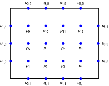
For example, suppose that the region is a rectangle with n=6 and m=5, and that the unknown values of u(x_i,y_j) at the twelve interior grid points are labeled p₁, p₂, ... ,p₁₂ and positioned in the grid as shown in the figure above. The Laplacian computational formula is applied at each of the interior grid points, and the result is the system A p = b of twelve linear equations:

\begin{align*} -4\,p_1 + p_2 + p_4 &= -u_{2,1} - u_{1,2} \\ p_1 -4\,p_2 + p_3 + p_5 &= -u_{3,1} , \\ \end{align*}

Example 1: Consider the Laplace equation in a square subject to the mixd boundary conditions

\begin{align*} &\mbox{Laplace equation:} \qquad &u_{xx} + u_{yy} &= 0 \qquad\mbox{for } -1 < x < 1 \mbox{ and } -1 < y < 1, \\ &\mbox{Dirichlet boundary conditions on }x: \qquad &u(-1,y) &= 50 , \quad \mbox{and} \quad u(1,y) = 40, \\ &\mbox{Neumann boundary condition on }y: \qquad &u_y(x,0) &= 1 , \quad \mbox{and} \quad u_y (x,1) = -1, \\ &\mbox{Corner regularity condition:} && \mbox{function } u(x,y) \quad \mbox{is bounded at every corner point}. \end{align*}

■

Amir, M.J., Yaseen, M., Iqbal, R., Exact solutions of Laplace equation by differential transform method,

Return to Mathematica page
Return to the main page (APMA0340)
Return to the Part 1 Matrix Algebra
Return to the Part 2 Linear Systems of Ordinary Differential Equations
Return to the Part 3 Non-linear Systems of Ordinary Differential Equations
Return to the Part 4 Numerical Methods
Return to the Part 5 Fourier Series
Return to the Part 6 Partial Differential Equations
Return to the Part 7 Special Functions

MATHEMATICA
TUTORIAL

under the terms of the GNU General Public License (GPL)

for the Second Course. Part VI: Numerical solutions of Laplace equation

Email: Prof. Vladimir Dobrushkin ()

Preface

Contents [hide]

Glossary

Numerical Solutions to Laplace Equations

MATHEMATICA TUTORIAL under the terms of the GNU General Public License (GPL) for the Second Course. Part VI: Numerical solutions of Laplace equation

Email: Prof. Vladimir Dobrushkin ()

Preface

Contents [hide]

Glossary

Numerical Solutions to Laplace Equations

MATHEMATICA
TUTORIAL

under the terms of the GNU General Public License (GPL)

for the Second Course. Part VI: Numerical solutions of Laplace equation