Preface
This section as well others related to it gives an introduction to nonlinear motion that is observed in many applications. Linear model is valid only in the very small amplitude approximations that a one-dimensional system trapped in the neighborhood of a point of stable equlibrium, which leads to a simple harmonic oscillator. Injection of energy into such a system increases the amplitude of its oscillations, causing the particle to begin to explore the completely different phenomenon that we observe for a simple idealized spring. Therefore, this section can be considered as an introduction to the theory of nonlinear oscillations and related topics.
To make exposition relatively simple and understandable at undergraduate level, we mostly work with some examples utilizing software. The reader should anticipate that numerical methods will play more prominent role in our qualitative analysis.
Return to computing page for the first course APMA0330
Return to computing page for the second course APMA0340
Return to Mathematica tutorial for the first course APMA0330
Return to Mathematica tutorial for the second course APMA0340
Return to the main page for the first course APMA0330
Return to the main page for the second course APMA0340
Return to Part III of the course APMA0340
Introduction to Linear Algebra with Mathematica
Glossary
Spring-mass system
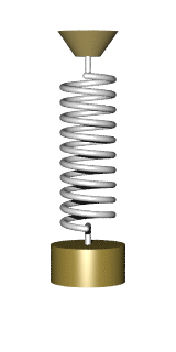 Consider a simple system consisting of a spring and attached to it a single
mass m. Suppose that the mass is put into motion my stretching it and
applying some impulse. Assuming its one dimensional motion, we choose
rectangular coordinates so that the origin x = 0 corresponds to its
stable equilibrium position (where the object would stay at rest if it was
released at rest). Once released, the restoring force causes the mass to move
back toward its stable equilibrium position, where the net force on it is zero.
However, by the time the mass gets there, it gains momentum and continues to
move through, producing the opposite deformation. It is then forced to the
opposite through equilibrium, and the process is repeated until dissipative
forces (e.g., friction) dampen the motion.
Consider a simple system consisting of a spring and attached to it a single
mass m. Suppose that the mass is put into motion my stretching it and
applying some impulse. Assuming its one dimensional motion, we choose
rectangular coordinates so that the origin x = 0 corresponds to its
stable equilibrium position (where the object would stay at rest if it was
released at rest). Once released, the restoring force causes the mass to move
back toward its stable equilibrium position, where the net force on it is zero.
However, by the time the mass gets there, it gains momentum and continues to
move through, producing the opposite deformation. It is then forced to the
opposite through equilibrium, and the process is repeated until dissipative
forces (e.g., friction) dampen the motion.
Due to various sources of nonlinearities, micro/nano-electro-mechanical-system (MEMS/NEMS) resonators present highly nonlinear behaviors including softening- or hardening-type frequency responses, bistability, chaos, etc. The general Duffing equation with quadratic and cubic nonlinearities serves as a characterizing model for a wide class of MEMS/NEMS resonators as well as lots of other engineering and physical systems.
The simplest oscillations occur when the restoring force is directly proportional to displacement. The name that was given to this relationship between force and displacement is Hooke’s law: \( f(x) = k\, x . \) Here, f is the restoring force, x(t) is the displacement from equilibrium or deformation at time t, and k is a constant related to the difficulty in deforming the system (often called the spring constant or force constant), with units of newtons per meter (N/m). For example, k is directly related to Young’s modulus when we stretch a string. Then Newton's second law yields
Multiplying the main equation \( m\,\ddot{x} + f(x) = 0 \) by the velocity \( \dot{x} = {\text d}x/{\text d}t , \) we obtain
The above expansion cannot be always true because the potential energy can be represented by a piecewise continuous function for which the Taylor series expansion is not valid. Moreover, even when such an expansion is possible, there are cases where the coefficient of the quadratic term vanishes and the series starts with a term higher than the second order.
Let us return to the string-mass problem when the potential energy retains the Taylor series expansion. Then such system can eb modeled by the following initial value problem:
if D > 0 and Exx = D > 0, then E has a local minimum;
if D < 0, then E has a a saddle point at (x0, y0).
If D = 0, the test is inconclusive.
The above system of differential equations always thas the critical point at the origin. Since its Jacobian
We can reduce the spring-mass differential equation \( \ddot{x} + x + a_2 x^2 + a_3 x^3 + \cdots + a_n x^n =0 \) to a separable differential equation of the first order using substitution: \( \dot{x} = 1/y . \) This yields
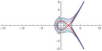
Example: We consider the pendulum equation and its two approximations:
q3 = ContourPlot[{p^2 + x^2 - x^3/3 == 3}, {x, -15, 10}, {p, -6, 6}, AspectRatio -> Automatic, Axes -> True, Frame -> False, ClippingStyle -> Automatic, ContourLabels -> True]
q2 = ContourPlot[{p^2 + x^2 - x^3/3 == 2}, {x, -15, 10}, {p, -6, 6}, AspectRatio -> Automatic, Axes -> True, Frame -> False, ClippingStyle -> Automatic, ContourLabels -> True]
q1 = ContourPlot[{p^2 + x^2 - x^3/3 == 1}, {x, -15, 10}, {p, -6, 6}, AspectRatio -> Automatic, Axes -> True, Frame -> False, ClippingStyle -> Automatic, ContourLabels -> True]
q43 = ContourPlot[{p^2 + x^2 - x^3/3 == 4/3}, {x, -15, 10}, {p, -6, 6}, AspectRatio -> Automatic, Axes -> True, Frame -> False, ClippingStyle -> Automatic, ContourLabels -> True, ColorFunction -> Hue]
q05 = ContourPlot[{p^2 + x^2 - x^3/3 == 0.5}, {x, -15, 10}, {p, -6, 6}, AspectRatio -> Automatic, Axes -> True, Frame -> False, ClippingStyle -> Automatic, ContourLabels -> True]
Show[q05, q1, q43, q2, q3, q4]
- Fay, T.H. and Joubert, S.V., Energy and nonsymmetric nonlinear spring, International Journal of Mathematical Education in Science and Technology, 1999, Vol. 30, No. 6, pp. 889--902; https://doi.org/10.1080/002073999287554
- Kovacic, I. and Brennan, M.J., The Duffing equation, nonlinear oscillators and their behavior 2011, Joun Wiley & Sons.
- Liao, S. Beyond perturbation introduction to homotopy analysis method, 2003, CRC Press.
- Main, I.G., Vibrations and waves in physics 1993, Cambridge University Press
- Olabode, D.L., Lamboni, B., Orou, J.B.C., Active Control of Chaotic Oscillations in Nonlinear Chemical Dynamics, JAMP. 2019, Vol. 7, No. 3, doi: 10.4236/jamp.2019.73040
- Oliveira, A.R.E., History of Krylov-Bogoliubov-Mitropolsky Methods of Nonlinear Oscillations, doi: 10.4236/ahs.2017.61003
- Sarafian, H., Dynamic Dipole-Dipole Magnetic Interaction and Damped Nonlinear Oscillations, JEMAA, 2009, Vol. 1, No. 4, doi: 10.4236/jemaa.2009.14030
- Sarafian, H., Nonlinear Oscillations of a Magneto Static Spring-Mass, JEMAA, 2011, Vol. 3, No. 5, doi: 10.4236/jemaa.2011.35022
Return to Mathematica page
Return to the main page (APMA0340)
Return to the Part 1 Matrix Algebra
Return to the Part 2 Linear Systems of Ordinary Differential Equations
Return to the Part 3 Non-linear Systems of Ordinary Differential Equations
Return to the Part 4 Numerical Methods
Return to the Part 5 Fourier Series
Return to the Part 6 Partial Differential Equations
Return to the Part 7 Special Functions