Preface
This section provides some analysis of spring-mass systems under quadratic restoring force.
Return to computing page for the first course APMA0330
Return to computing page for the second course APMA0340
Return to Mathematica tutorial for the first course APMA0330
Return to Mathematica tutorial for the second course APMA0340
Return to the main page for the first course APMA0330
Return to the main page for the second course APMA0340
Return to Part III of the course APMA0340
Introduction to Linear Algebra with Mathematica
Glossary
Quadratic damping
When modeling a spring-mass system, we usually need to take into account resistance forces acting on a spring and a mass (friction). These forces are typically noninear and their modeling requires variable approximations at different stages. Previously, we discussed viscous damping and cubic restoring force in the Duffing model. In this section, we consider the spring's restoring force that is only mildly nonlinear. This leads to an even function (quadratic) as a restoring force and corresponding differential equation
|
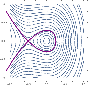
As the phase portrate shows, the origin is a center, but P is a saddle point. We plot the phase portrate for the equation
\[
\ddot{x} + x +3\,x^2 = 0 .
\tag{1.2}
\]
along with the separatrix:
sp = StreamPlot[{v, -x - 2*x^2}, {x, -1, 1}, {v, -1, 1},
StreamStyle -> Thick];
s1 = NDSolve[{x''[t] + x[t] + 2*x[t]^2 == 0, x[0] == 0.2495, x'[0] == 0.0198}, x, {t, -14, 14}]; pp1 = ParametricPlot[Evaluate[{x[t], x'[t]} /. s1], {t, 0, 13}, PlotRange -> {{-1, 1}, {-1, 1}}, PlotStyle -> {Thickness[0.01], Purple}]; mm1 = ParametricPlot[Evaluate[{x[t], x'[t]} /. s1], {t, 0, -13}, PlotRange -> {{-1, 1}, {-1, 1}}, PlotStyle -> {Thickness[0.01], Purple}]; Show[sp, pp1, mm1] |
|
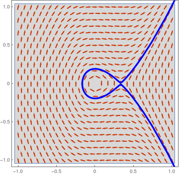
We plot the phase portrate for the equation
\[
\ddot{x} + x -3\,x^2 = 0 .
\tag{1.2}
\]
along with the separatrix:
s3 = NDSolve[{x''[t] + x[t] - 3*x[t]^2 == 0, x[0] == -0.167,
x'[0] == 0}, x, {t, -14, 14}];
vp = VectorPlot[{v, -x + 3*x^2}, {x, -1, 1}, {v, -1, 1}, PlotTheme -> "Web", RegionFillingStyle -> Gray, VectorPoints -> Fine]; pp3 = ParametricPlot[Evaluate[{x[t], x'[t]} /. s3], {t, 0, 13}, PlotRange -> {{-1, 1}, {-1, 1}}, PlotStyle -> {Thickness[0.01], Blue}]; mm3 = ParametricPlot[Evaluate[{x[t], x'[t]} /. s3], {t, 0, -13}, PlotRange -> {{-1, 1}, {-1, 1}}, PlotStyle -> {Thickness[0.01], Blue}]; Show[vp, pp3, mm3] |
■
s1 = NDSolve[{x''[t] + x[t] + x'[t]/3 - 3*x[t]^2 == 0, x[0] == 0.4, x'[0] == -0.0609}, x, {t, -10, 10}];
s2 = NDSolve[{x''[t] + x[t] + x'[t]/3 - 3*x[t]^2 == 0, x[0] == 0.25, x'[0] == -0.463}, x, {t, -10, 10}];
pp1 = ParametricPlot[Evaluate[{x[t], x'[t]} /. s1], {t, 0, 10}, PlotRange -> {{-1, 1}, {-1, 1}}, PlotStyle -> {Thickness[0.01], Purple}];
pp2 = ParametricPlot[Evaluate[{x[t], x'[t]} /. s2], {t, 0, 7.0}, PlotRange -> {{-1, 1}, {-1, 1}}, PlotStyle -> {Thickness[0.01], Purple}];
mm1 = ParametricPlot[Evaluate[{x[t], x'[t]} /. s1], {t, 0, -10}, PlotRange -> {{-1, 1}, {-1, 1}}, PlotStyle -> {Thickness[0.01], Purple}];
Show[sp, pp1, mm1, pp2]
s1 = NDSolve[{x''[t] + x[t] + x'[t]/3 + 3*x[t]^2 == 0, x[0] == -0.4, x'[0] == -0.0609}, x, {t, -10, 10}];
s2 = NDSolve[{x''[t] + x[t] + x'[t]/3 + 3*x[t]^2 == 0, x[0] == -0.25, x'[0] == 0.463}, x, {t, -10, 10}];
pp1 = ParametricPlot[Evaluate[{x[t], x'[t]} /. s1], {t, 0, 10}, PlotRange -> {{-1, 1}, {-1, 1}}, PlotStyle -> {Thickness[0.01], Purple}];
pp2 = ParametricPlot[Evaluate[{x[t], x'[t]} /. s2], {t, 0, 7.0}, PlotRange -> {{-1, 1}, {-1, 1}}, PlotStyle -> {Thickness[0.01], Purple}];
mm1 = ParametricPlot[Evaluate[{x[t], x'[t]} /. s1], {t, 0, -10}, PlotRange -> {{-1, 1}, {-1, 1}}, PlotStyle -> {Thickness[0.01], Purple}];
Show[sp, pp1, mm1, pp2]
|
|
|
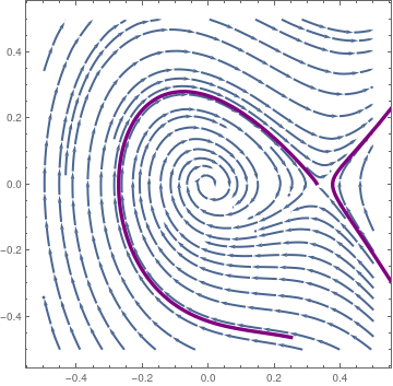
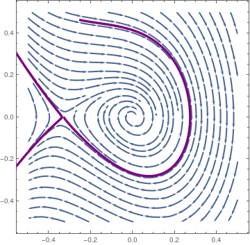
| Phase portrait for \( \ddot{x} + x + \frac{1}{3}\,\dot{x} -3\,x^2 = 0 , \) wityh separatrix. | Phase portrait for \( \ddot{x} + x + \frac{1}{3}\,\dot{x} +3\,x^2 = 0 , \) with separatrix. |
■
To analyze Eq.\eqref{EqQuadratic.1}, we convert it to the system of first order ODEs:
The eigenvalues of matrix J(−1/ε, 0) are \( \displaystyle \lambda = \frac{1}{2} \left( -k \pm \sqrt{k^2 + 4} \right) . \) Therefore, it is a saddle point because eigenvalues are real and of different sign.
Viscous damping is a mathematical convenience and its use results from its simplicity. However, it is not completely accurate, especially for velocities that are large. For velocities that are larger, the frictional force is probably proportional to the square of the velocity, as opposed to a linear relationship like in viscous damping. For larger velocities, quadratic damping is used. Quadratic damping is more realistic and applicable to many models, including motion through fluids and gases. For example modelling the drag on a bird flying through strong winds. For quadratic damping, because it always opposes the direction of the motion, there is a jump discontinuity when velocity equals zero.
To calculate the maximum amplitudes of the oscillations of quadratically damped harmonic oscillators and quadratically damped pendulums, an approach with energy is used. To start, the jump discontinuity is ignored and we find a generalized energy function for
Inhomogeneous equation
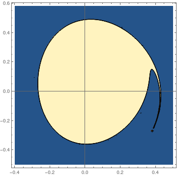
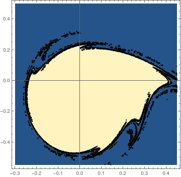
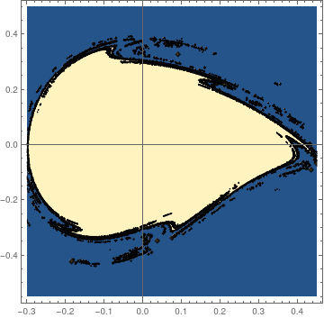
To get an idea of what responses are available, we begin with some examples that have interesting trajectories in the phase plane. The first example is that with a harmonic solution having a typical harmonic trajectory.
|
pfun = ParametricNDSolveValue[{x''[t] +
2 x[t] - (3*x[t])^2/6 == (1/2)*Sin[t/5], x[0] == a, x'[0] == b},
x, {t, 0, 100}, {a, b}];
fun[a_?NumericQ, b_?NumericQ] := Module[{res}, res = Quiet[pfun[a, b]]; Boole[res["Domain"] === {{0., 100.}}]]; plot = ContourPlot[fun[a, b], {a, -0.4, 0.5}, {b, -0.5, 0.58}, PlotPoints -> 50, MaxRecursion -> 3, Axes -> True, AxesOrigin -> {0, 0}] |
|
| Domain of stability. | Mathematica code. |
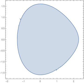
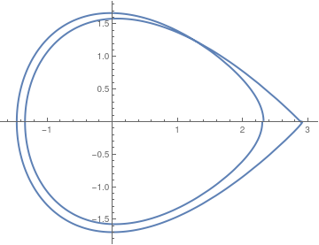
Now we consider slightly different equation
|
pfun = ParametricNDSolveValue[{3 x''[t] + 3 x[t] - (x[t])^2 == (1/3)*
Sin[t/8], x[0] == a, x'[0] == b}, x, {t, 0, 100}, {a, b}];
fun[a_?NumericQ, b_?NumericQ] := Module[ {res}, (* determine if domain is valid or invalid and return 1 or 0 respectively *) res = Quiet[pfun[a, b]]; Boole[res["Domain"] === {{0., 100.}}] ]; regionplot = RegionPlot[fun[a, b] >= 1, {a, -2.0, 2.5}, {b, -1.7, 1.7}] |
|
| Domain of stability. | Mathematica code. |
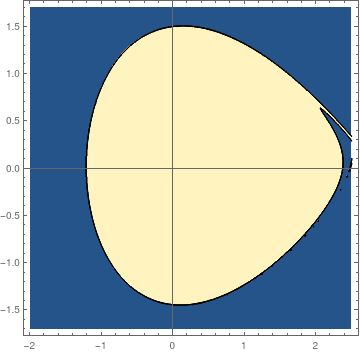
For another input sine function, we obtain almost the same stability domain. However, for the following equation
|
pfun = ParametricNDSolveValue[{3 x''[t] +
3 x[t] - (x[t])^2 == (1/3)*Cos[t/8] + (1/3)*Sin[t/8], x[0] == a,
x'[0] == b}, x, {t, 0, 100}, {a, b}];
fun[a_?NumericQ, b_?NumericQ] := Module[{res}, res = Quiet[pfun[a, b]]; Boole[res["Domain"] === {{0., 100.}}]]; plot = ContourPlot[fun[a, b], {a, -2.0, 2.5}, {b, -1.7, 1.7}, PlotPoints -> 50, MaxRecursion -> 3, Axes -> True, AxesOrigin -> {0, 0}] |
|
| Domain of stability. | Mathematica code. |
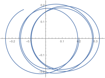
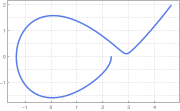
We plot some typical trajectories.
ParametricPlot[Evaluate[{x[t], x'[t]} /. sol2], {t, 0, 30}, PlotStyle -> Thick]
ParametricPlot[Evaluate[{x[t], x'[t]} /. sol2], {t, 0, 30}, PlotStyle -> Thick]
ParametricPlot[Evaluate[{x[t], x'[t]} /. sol2], {t, 0, 13}, PlotTheme -> "Business"]
|
|
|
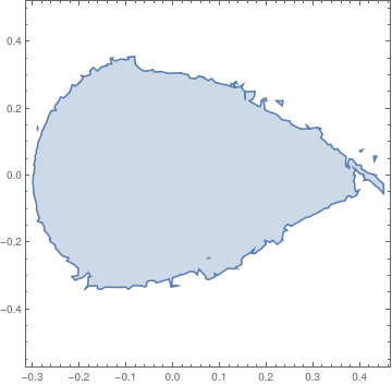
We use manipulate command to determine the boundary of stability domain for another equation:
fun[a_?NumericQ, b_?NumericQ] := Module[ {res}, (* determine if domain is valid or invalid and return 1 or 0 respectively *) res = Quiet[pfun[a, b]]; Boole[res["Domain"] === {{0., 100.}}] ];
regionplot = RegionPlot[fun[a, b] >= 1, {a, -0.3, 0.45}, {b, -0.55, 0.5}];
mesh = BoundaryDiscretizeGraphics[regionplot]
Manipulate[ ListPlot[coord[[1 ;; n]], PlotRange -> {{-0.3, 0.45}, {-0.55, 0.5}}], {{n, 50}, 1, Length[coord], 1}]
|
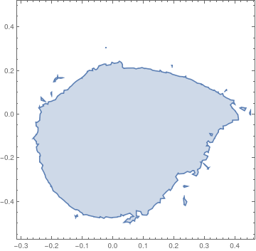
|
On the other hand, the stability domain for the differential equation with cosine driving function is
|
|
■
Nonlinearity is typically introduced by assuming that the spring’s restoring force is nonlinear and perhaps the most common form is that of the Duffing spring equation
Return to Mathematica page
Return to the main page (APMA0340)
Return to the Part 1 Matrix Algebra
Return to the Part 2 Linear Systems of Ordinary Differential Equations
Return to the Part 3 Non-linear Systems of Ordinary Differential Equations
Return to the Part 4 Numerical Methods
Return to the Part 5 Fourier Series
Return to the Part 6 Partial Differential Equations
Return to the Part 7 Special Functions