Preface
This section presents analysis of hard spring model, derived by Georg Duffing (1861–1944) in 1918.
Return to computing page for the second course APMA0340
Return to Mathematica tutorial for the first course APMA0330
Return to Mathematica tutorial for the second course APMA0340
Return to the main page for the first course APMA0330
Return to the main page for the second course APMA0340
Return to Part III of the course APMA0340
Introduction to Linear Algebra
Glossary
Undriven Hard Spring
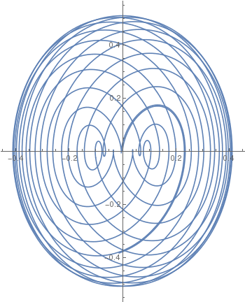
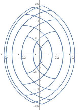
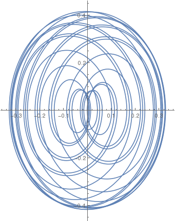
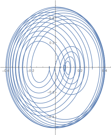
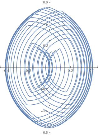
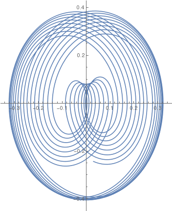
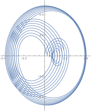
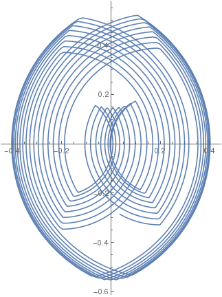
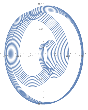
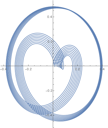
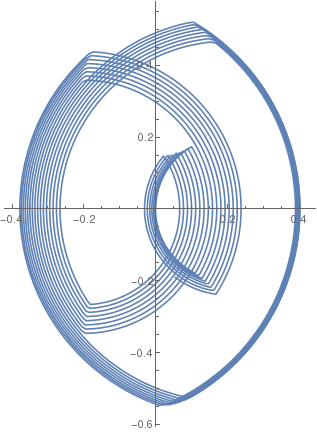
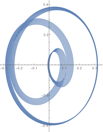
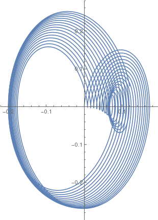
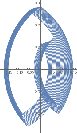
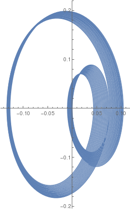
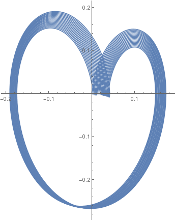
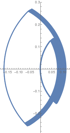
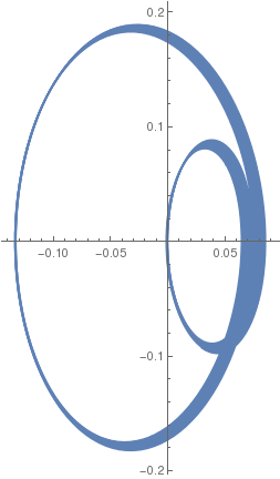
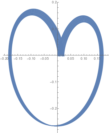
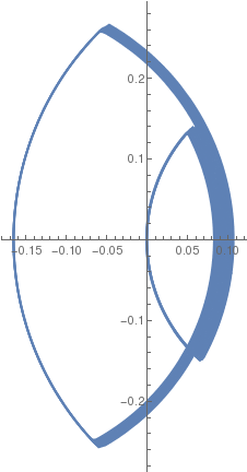
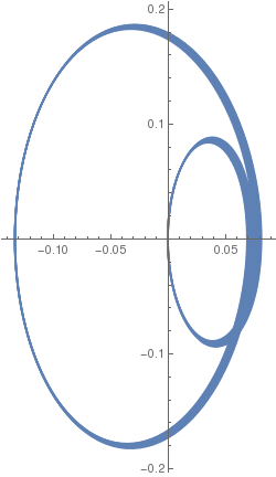
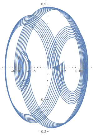
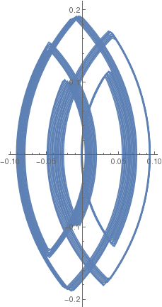
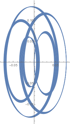
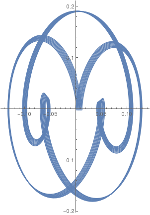
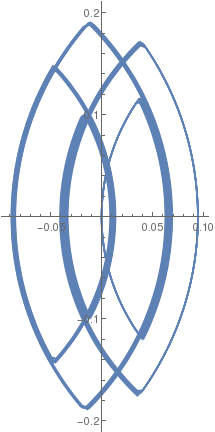
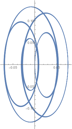
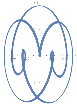
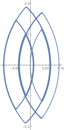
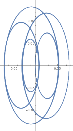
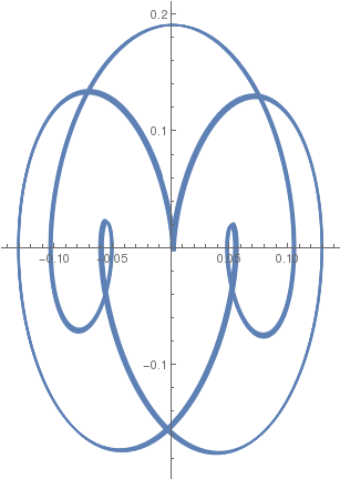
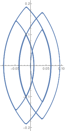
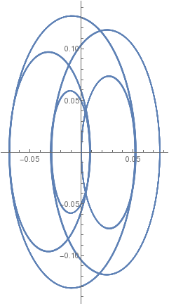
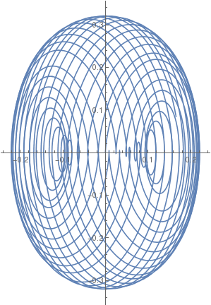
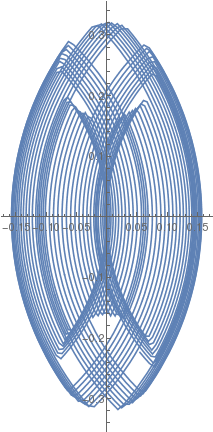
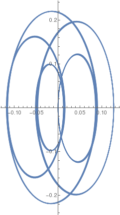
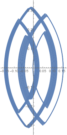
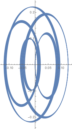
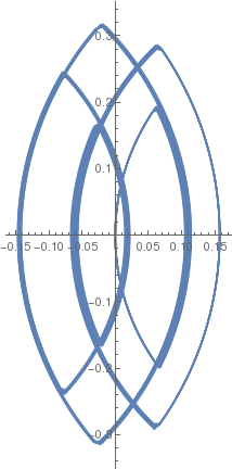
Undamped Driven Hard Spring
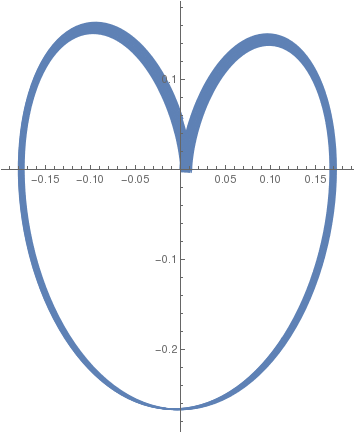
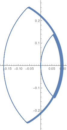
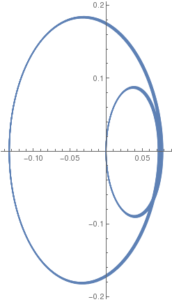
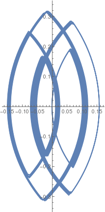
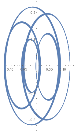
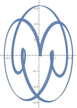
We consider second-order differential equations of the general form \( \ddot{x} + f\left( x, \dot{x} \right) = F(t) , \) when F(t) is a periodic function, of which we consider three of them:
| F = (1/5) sign(sin(1.5 t)) | F = (1/5) sin(1.5 t) | F = (1/5) sign(cos(1.5 t)) | F = (1/5) cos(1.5 t) | |
|---|---|---|---|---|
| β = 1 | 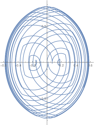 |
 |
 |
 |
| β = 1/3 | 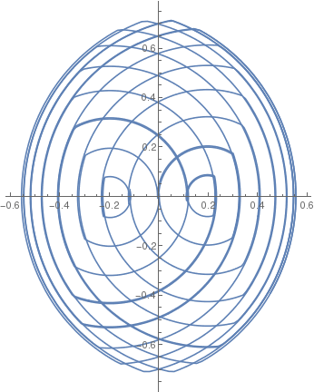 |
 |
 |
 |
| β = 1/5 | 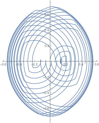 |
 |
 |
 |
| β = 1/10 | 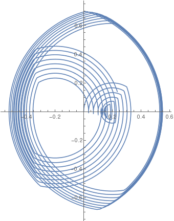 |
 |
 |
 |
| F = (1/5) sign(sin(2.0 t)) | F = (1/5) sin(2.0 t) | F = (1/5) sign(cos(2.0 t)) | F = (1/5) cos(2.0 t) | |
|---|---|---|---|---|
| β = 1 | 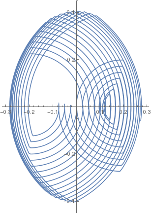 |
 |
 |
 |
| β = 1/3 | 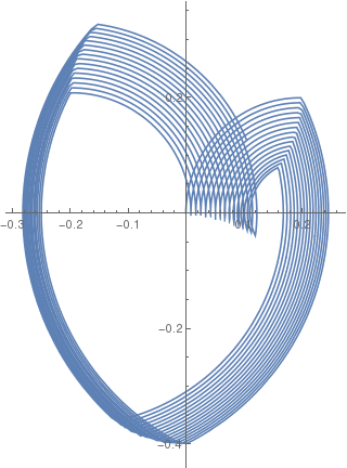 |
 |
 |
 |
| β = 1/5 | 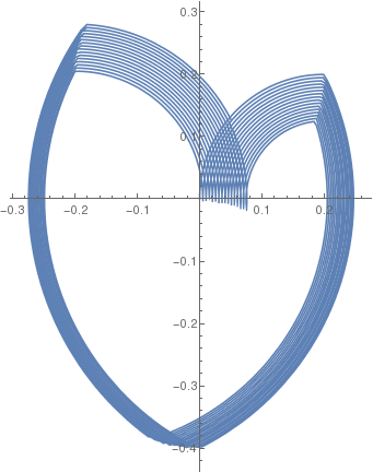 |
 |
 |
 |
| β = 1/10 | 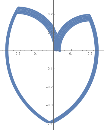 |
 |
 |
 |
| F = (1/5) sign(sin(2.5 t)) | F = (1/5) sin(2.5 t) | F = (1/5) sign(cos(2.5 t)) | F = (1/5) cos(2.5 t) | |
|---|---|---|---|---|
| β = 1 | 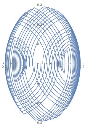 |
 |
 |
 |
| β = 1/3 | 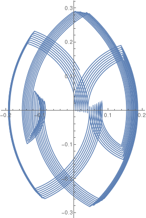 |
 |
 |
 |
| β = 1/5 | 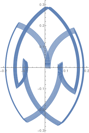 |
 |
 |
 |
| β = 1/10 | 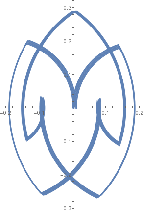 |
 |
 |
 |
| F = (1/3) sign(sin(2.5 t)) | F = (1/3) sin(2.5 t) | F = (1/3) sign(cos(2.5 t)) | F = (1/3) cos(2.5 t) | |
|---|---|---|---|---|
| β = 1 | 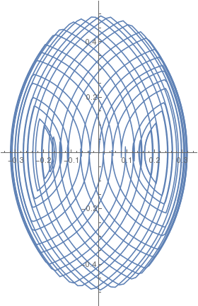 |
 |
 |
 |
| β = 1/3 | 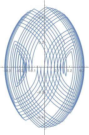 |
 |
 |
 |
| β = 1/5 | 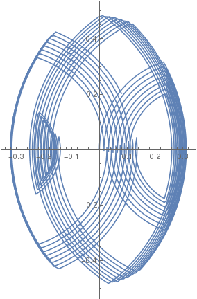 |
 |
 |
 |
| β = 1/10 | 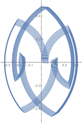 |
 |
 |
 |
Nonhomogeneous Initial Value Problem
Frequency Response
The forced Duffing oscillator with cubic nonlinearity is described by the following ordinary differential equation:
The frequency response of this oscillator describes the amplitude z of steady state response of the equation (i.e. x(t)) at a given frequency of excitation \omega . For a linear oscillator with \beta =0, the frequency response is also linear. However, for a nonzero cubic coefficient, the frequency response becomes nonlinear. Depending on the type of nonlinearity, the Duffing oscillator can show hardening, softening or mixed hardening–softening frequency response. Anyway, using the homotopy analysis method or harmonic balance, one can derive a frequency response equation in the following form:
Damped Driven Hard Spring
- Brennan, M.J.; Kovacic, I.; Carrella, A.; Waters, T.P., On the jump-up and jump-down frequencies of the Duffing oscillator, Journal of Sound and Vibration, 2008, Vol. 318, Issues 4–5, pp. 1250--1261. doi:10.1016/j.jsv.2008.04.032
- Duffing, G., Erzwungene Schwingungen bei veränderlicher Eigenfrequenz und ihre technische Bedeutung [Forced oscillations with variable natural frequency and their technical relevance] (in German), 1918, Heft 41/42, pp. 134.
- Fay, T.H., the forced hard spring equation, International Journal of Mathematical Education in Science and Technology, 2006, Vol. 37, No. 2, pp. 187--200; doi: 10.1080/00207390500285735
- Jordan D.W. and Smith P., Nonlinear Ordinary Differential Equations An introduction for Scientists and Engineers, fourth edition, Oxford University Press, Oxford, 2007.
- Liao S (2003) Beyond perturbation introduction to homotopy Analysis method. CRC Press
- Liao S (2004a) On the homotopy analysis method for nonlinear problems. Appl Math Comput 147:499–513. doi: 10.1016/S0096-3003(02)00790-7
- Liao S (2004b) An analytic approximate approach for free oscillations of self-excited systems. Int J Non Linear Mech 39:271–280
- Liao S (2009) Notes on the homotopy analysis method: some definitions and theorems. Commun Nonlinear Sci Numer Simul 14:983–997. doi: 10.1016/j.cnsns.2008.04.013
- Liao S (2012) Homotopy Analysis Method in Nonlinear Differential Equations. Springer
- Kovacic, I.; Brennan, M.J., eds. (2011), The Duffing Equation: Nonlinear Oscillators and their Behaviour, Wiley, 392 pp., ISBN 978-0-470-71549-9
- Tajaddodianfar, F.; Yazdi, M.R.H.; Pishkenari, H.N., Nonlinear dynamics of MEMS/NEMS resonators: analytical solution by the homotopy analysis method, Microsystem Technologies, 2016, doi:10.1007/s00542-016-2947-7
- Duffing equation, WikiVisually
Return to Mathematica page
Return to the main page (APMA0340)
Return to the Part 1 Matrix Algebra
Return to the Part 2 Linear Systems of Ordinary Differential Equations
Return to the Part 3 Non-linear Systems of Ordinary Differential Equations
Return to the Part 4 Numerical Methods
Return to the Part 5 Fourier Series
Return to the Part 6 Partial Differential Equations
Return to the Part 7 Special Functions