Return to computing page for the first course APMA0330
Return to computing page for the second course APMA0340
Return to Mathematica tutorial for the first course APMA0330
Return to Mathematica tutorial for the second course APMA0340
Return to the main page for the first course APMA0330
Return to the main page for the second course APMA0340
Return to Part III of the course APMA0340
Introduction to Linear Algebra with Mathematica
Glossary
Pendulum Equations
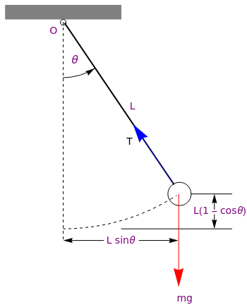
A simple pendulum consists of a single point of mass m (bob) attached to a rod (or wire) of length \( \ell \) and of negligible weight. We denote by θ the angle measured between the rod and the vertical axis, which is assumed to be positive in counterclockwise direction. We consider the simple pendulum that is characterized by the following assumptions:
- The bob is free to move within a plane (so we consider only two-dimensional oscillations).
- The system is conservative, so the pendulum rotates in a vacuum and friction in the pivot is negligible.
- The bob of mass m is attached to one end of a rigid, but weightless rod of length ℓ, which is assumed to be constant during the pendulum motion. The other end of the rod (or rigid spring) is supported at the pivot.
f[s_Circle] := s /. Circle[a_, r_, {start_, end_}] :> ({s, Arrow[{# - r/10^6 {-Sin@end, Cos@end}, #}]} &[ a + r {Cos@end, Sin@end}])
polygon = Polygon[{{-1, 0}, {1, 0}, {1, 1/4}, {-1, 1/4}}];
top = Graphics[{Gray, polygon}];
circle1 = Graphics[Circle[{0, -1/20}, 1/20]];
circle2 = Graphics[Circle[{2, -3}, 1/5]];
circle3 = Graphics[{Dashed, Circle[{0, 0}, 3.6, {-1.57, -1.0}]}];
line1 = Graphics[{Dashed, Line[{{0, -1/20}, {0, -3.8}}]}];
line2 = Graphics[{Thick, Line[{{0.03, -0.07}, {1.9, -2.83}}]}];
arrow = Graphics[{Red, Arrowheads[0.08], Arrow[{{1.986, -3.0}, {1.986, -4.6}}]}]; line3 = Graphics[{Line[{{2.2, -3.8}, {2.9, -3.8}}]}];
arrow2a = Graphics[{Arrowheads[0.04], Arrow[{{0.7, -3.8}, {0, -3.8}}]}];
arrow2b = Graphics[{Arrowheads[0.04], Arrow[{{1.3, -3.8}, {1.98, -3.8}}]}];
text1 = Graphics[ Text[Style["L sin\[Theta]", FontSize -> 14, Purple], {1.0, -3.8}]];
text2 = Graphics[ Text[Style["mg", FontSize -> 14, Purple], {2.1, -4.8}]];
line3 = Graphics[{Line[{{1.0, -3.6}, {2.9, -3.6}}]}];
line4 = Graphics[{Line[{{2.2, -3.0}, {2.9, -3.0}}]}];
text3 = Graphics[ Text[Style["L(1 - cos\[Theta])", FontSize -> 14, Purple], {2.7, -3.3}]];
arrow3a = Graphics[{Arrowheads[0.04], Arrow[{{2.6, -3.35}, {2.6, -3.6}}]}];
arrow3b = Graphics[{Arrowheads[0.04], Arrow[{{2.6, -3.27}, {2.6, -3.0}}]}];
text4 = Graphics[ Text[Style["L", FontSize -> 14, Purple], {1.2, -1.5}]];
text5 = Graphics[ Text[Style["\[Theta]", FontSize -> 16, Purple], {0.2, -0.7}]];
text6 = Graphics[ Text[Style["O", FontSize -> 14, Purple], {-0.16, -0.2}]];
textT = Graphics[ Text[Style["T", FontSize -> 14, Black], {1.15, -2.1}]];
arrowT = Graphics[{Blue, Arrowheads[0.08], Arrow[{{1.88, -2.8}, {1.2, -1.8}}]}];
Show[top, circle1, circle2, circle3, line1, line2, line3, arrow, arrow2a, arrow2b, text1, text2, line4, text3, arrow3a, arrow3b, text4, text5, text6, arrowT, textT, arc]
|
The modeling of the motion is greatly simplified when the given body (bob) is considered essentially as a point particle. The position of the bob is described by the angle θ between the rod and the downward equilibrium vertical position, with the counterclockwise direction taken as positive. The only force acting on the pendulum is the gravitational force m g, acting downward, where g denotes the acceleration due to gravity. The position of the bob can be determined in Cartesian coordinates as
\[
x = \ell \,\sin \theta , \qquad y = -\ell\,\cos\theta ,
\]
where the origin is taken at the pivot and the positive vertical direction is upward.
Using \( {\cal L} = \mbox{K} - \Pi , \) the
Lagrangian,
which is the difference of the kinetic energy K and the potential
energy Π of the system, we have
\[
\frac{\text d}{{\text d}t} \,\frac{\partial {\cal L}}{\partial \dot{\theta}}
= \frac{\partial {\cal L}}{\partial \theta} .
\]
|
With the kinetic energy expressed via the angular displacement θ
Further simplification is available by normalization, which leads to \( \omega = 1 \) and we get
Example: The swinging mass m has a kinetic energy of \( m \ell^2 \left( {\text d}\theta /{\text d}t \right)^2 /2 \) and a potential energy of \( mg\ell\left( 1 - \cos \theta \right) ; \) the potential energy is zero for θ = 0. Let θM denote the maximum amplitude of the pendulum. Since dθ/dt = 0 at θ = θM, conservation of energy gives
Pendulum Equation with Resistance
We convert the pendulum equation with resistance
Pendulum with a ball
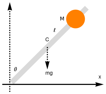
Let us consider a rod of length ℓ of mass m with attached ball of mass M at a distance L from the pivot.
|
rod = Graphics[{LightGray,
Polygon[{{0.1, 0}, {0, 0.1}, {2.0, 2.1}, {2.1, 2.0}}]}];
ball = Graphics[{Orange, Disk[{1.75, 1.75}, 0.25]}]; ar3 = Graphics[{Black, Dashed, Thickness[0.01], Arrowheads[0.08], Arrow[{{1, 1}, {1, 0.4}}]}]; ar = Graphics[{Black, Thickness[0.01], Arrowheads[0.08], Arrow[{{-0.2, 0}, {2.5, 0}}]}]; ar2 = Graphics[{Black, Dashed, Thickness[0.01], Arrowheads[0.08], Arrow[{{0, -0.2}, {0, 2.2}}]}]; tl = Graphics[{Black, Text[Style["\[ScriptL]", 18, FontFamily -> "Mathematica1"], {1.2, 1.45}]}]; tx = Graphics[{Black, Text[Style["x", 18], {2.4, 0.2}]}]; tm = Graphics[{Black, Text[Style["M", 18, FontFamily -> "Mathematica1"], {1.4, 1.75}]}]; t1 = Graphics[{Black, Text[Style["C", 18], {1.0, 1.2}]}]; t2 = Graphics[{Black, Text[Style["\[Theta]", 18], {0.15, 0.4}]}]; t3 = Graphics[{Black, Text[Style["mg", 18], {1.05, 0.3}]}]; Show[rod, ar, ar2, ar3, tx, tl, tm, t1, t2, t3, ball] |
|
| Rigid pendulum with a ball. | Mathematica code |
To analyze the problem of falling meterstick of length ℓ with attached heavy weight at a distance L from the pivot, we use the tourque equation:
Spherical Pendulum
Consider the motion under gravity of a bob of mass m attached to a fixed point by an inextensible massless rod of length ℓ. The bob is free to move on a sphere of radius ℓ. Using spherical coordinates (angles) θ and ϕ as the generalized coordinates, the kinetic and potential energies become
Applications
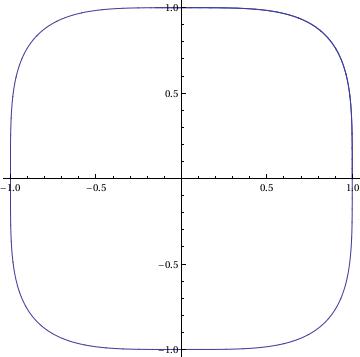
G[x_, y_] := x^3;
sol = NDSolve[{x'[t] == F[x[t], y[t]], y'[t] == G[x[t], y[t]],
x[0] == 1, y[0] == 0}, {x, y}, {t, 0, 3*Pi},
WorkingPrecision -> 20]
ParametricPlot[Evaluate[{x[t], y[t]}] /. sol, {t, 0, 3*Pi}]
{{x -> InterpolatingFunction[{{0, 9.4247779607693797154}}, <>],
y -> InterpolatingFunction[{{0, 9.4247779607693797154}}, <>]}}
Y[t_] := Evaluate[y[t] /. sol]
fns[t_] := {X[t], Y[t]};
len := Length[fns[t]];
Plot[Evaluate[fns[t]], {t, 0, 3*Pi}]
-
Vitt, A. (Aleksandr Adolʹfovich) and Gorelik, G. (Gabriel Simonovich), Oscillations of an Elastic Pendulum as an Example of the Oscillations of Two
Parametrically Coupled Linear Systems,
Journal of Technical Physics, 1933, vol. 3, pp. 294–307.
Its translation from the Russian in English by Lisa Shields with an introduction by Peter Lynch is available on the web:
http://copac.jisc.ac.uk/id/15694518?style=html
http://catalogue.nli.ie/Record/vtls000058645 -
P. Pokorny, Stability condition for vertical oscillation of 3-dim heavy spring elastic pendulum,
Regular and Chaotic Dynamics,
June 2008, Volume 13, Issue 3, pp 155--165.
https://link.springer.com/article/10.1134/S1560354708030027
http://old.vscht.cz/mat/Pavel.Pokorny/rcd/RCD155-color.pdf - Pendulum Wikipedia
- Pendulum Physics
- Lumen Physics: Pendulum
- Predicting the Future – An Intro to Models Described by Time Dependent Differential Equations by Christian J Howard.
- Salas, A.H. and Castillo, J.E., Exact Solution to Duffing Equation and the Pendulum Equation, Applied Mathematical Sciences, Vol. 8, 2014, no. 176, 8781 - 8789; http://dx.doi.org/10.12988/ams.2014.44243
- M. G. Olsson, Why does a mass on a spring sometimes misbehave?, American Journal of Physics, 44, Issue 12, 1211 (1976); https://doi.org/10.1119/1.10265
- Casey, J., Geometrical derivation of Lagrange’s equations for a system of particles, American Journal of Physics, 62(9) 836–847 (1994). https://doi.org/10.1119/1.17470
- Corey Zammit, Nirantha Balagopal, Zijun Li, Shenghao Xia, and Qisong Xiao, The dynamic of the elastic pendulum, Arizona.
- Qisong Xiao; Shenghao Xia; Corey Zammit; Nirantha Balagopal; Zijun Li, Dynamics of the Elastic Pendulum, Arizona.
- C. Madigan, The Spring Pendulum, MapleSoft.
- K. Craig, Pring-pendulum dynamic system, NYU, 2001.
Return to Mathematica page
Return to the main page (APMA0340)
Return to the Part 1 Matrix Algebra
Return to the Part 2 Linear Systems of Ordinary Differential Equations
Return to the Part 3 Non-linear Systems of Ordinary Differential Equations
Return to the Part 4 Numerical Methods
Return to the Part 5 Fourier Series
Return to the Part 6 Partial Differential Equations
Return to the Part 7 Special Functions