Return to computing page for the first course APMA0330
Return to computing page for the second course APMA0340
Return to Mathematica tutorial for the first course APMA0330
Return to Mathematica tutorial for the second course APMA0340
Return to the main page for the first course APMA0330
Return to the main page for the second course APMA0340
Return to Part VII of the course APMA0340
Introduction to Linear Algebra with Mathematica
Although Johann Bernoulli (1667--1748) came in 1694 to an equation that is a particular case of what we call now the Bessel equation, it was his son who actually introduced it.
Daniel Bernoulli (1700--1782) is generally credited with being the first to introduce the concept of Bessels functions in 1732 (Saint Petersburg). He used the function of zero order J0(x) as a solution to the problem of an oscillating
chain suspended at one end. He also discovered that the equation J0(x) = 0 has infinuitely many zeroes. In 1732 (Saint Petersburg), Leonhard Euler (1707--1783) employed Bessel functions of both zero and integral orders in an analysis of vibrations of a stretched membrane. He also found Maclaurin series for Jn(x) with integer values of n. Also, Leonhard showed that Bessel's function of half integer order can be expressed through elementary functions.
Bessel functions were used by Lagrange in 1770, in the theory of planetary motion, by Fourier in his theory of heat flow (1822), by Poisson in the theory of heat flow in spherical bodies (1823), and by Bessel, who studied these functions in detail around 1824. It was Lord Rayleigh who demonstrated that Bessel's
functions are particular cases of Laplace's functions in 1878. Watson (1966) provided the most comprehensive study of the Bessel functions. See Dutka's historical notes.
This section is about Bessel's equation and its solutions, known as Bessel functions or cylinder functions. The origin of the term cylinder is due to the fact that these functions are encountered in studying the boundary–value problems of potential theory for cylindrical coordi-nates.
The Bessel differential equation is the linear second-order ordinary differential equation given by
where ν is a real constant, called the order of the Bessel equation.
Eq.\eqref{EqBessel.1} has a regular singularity at x = 0.
Upon substitution \( y = u\, x^{-1/2} , \) it is reduced to the equation without first derivative:
The systematic analysis of solutions to equation \eqref{EqBessel.1} was conducted around 1817 by the German astronomer Friedrich Wilhelm Bessel (1784--1846) during an investigation of solutions of one of Kepler’s equations of planetary motion.
The Bessel function was the result of Bessel's study of a
problem of Kepler for determining the motion of three bodies moving under mutual gravita-
tion. In 1824, he incorporated Bessel functions in a study of planetary perturbations where
the Bessel functions appear as coefficients in a series expansion of the indirect perturbation
of a planet, that is the motion of the Sun caused by the perturbing body. It was likely
Lagrange’s work on elliptical orbits that first suggested to Bessel to work on the Bessel functions.
Bessel's equation \eqref{EqBessel.1} is a special case of a confluent hypergeometric equation. Since x = 0 is a regular singular point for the Bessel equation, one of its solution can be bounded at this point but another linearly independent solution should be unbounded. A generalized series for bounded solution of Bessel's equation was found in section of tutorial I.
It is a custom to separate bounded solutions from unbounded solutions of Bessel's equation. A bounded solution is usually denoted by Jν(x) and called the Bessel function of the first kind or just Bessel's function. All other bounded solutions of Eq.\eqref{EqBessel.1} are constant multiples of this function. On the other hand, an unbounded solution is refferred to as the Bessel function of the second kind. Their complex combination is called the Bessel function of the third kind or "Hunkel's function. Bessel functions of complex argument are referred to as the Kelvin functions.
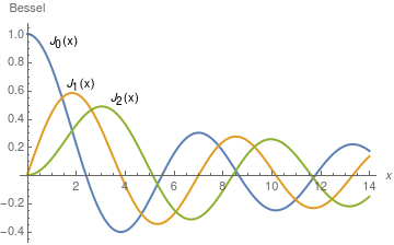
Bessel function of first kind
The Bessel function of first kind of order ν of real argument x is usually denoted by Jν(x). Its generalized series expansion was found previously (see section of tutorial I):
The notation Jz,n was first used by a Danish-born German astronomer Peter Hansen (1795--1874) in 1843 and subsequently by Oskar Xavier Schlömilch in 1857 and later modified to Jn(2z) by Watson (1922). Subsequent studies of Bessel functions included the works of Mathews in 1895, “A treatise
on Bessel functions and their applications to physics” written in collaboration with Andrew Gray. It was the first major treatise on Bessel functions in English and covered topics such as applications of Bessel functions to electricity, hydrodynamics and diffraction. In 1922, Watson first published his comprehensive examination of Bessel functions “A Treatise on the Theory of Bessel Functions”.
Since Bessel's equation \eqref{EqBessel.1} has a singular point at the origin, initial conditions are not specified for it because they do not identify a unique solution of the equation and cannot be chosen arbitrary. Nevertheless, they make sense for a bounded solution although the initial conditions for the function y(x) and its derivative at x = 0 are coupled (meaning that one of them forced another one to have a specific value). Then to find a bounded solution of Eq.\eqref{EqBessel.1} we apply the Laplace transformation:
Using notation \( \omega = \lambda + \sqrt{\lambda^2 +1} , \) we apply the inverse Laplace transform to determine a bounded solution to Bessel's equation:
where P.V. stands for Principle Value regularization and j is the unit vector in positive verstical direction on the complex plane, so j² = −1. This integral is named after Russian mathematician Nikolay Sonin (1849--1915). Upon setting \( \omega = e^{{\bf j}\zeta} , \) the Sonin integral is expressed as
This leads to series representation \eqref{EqBessel.2} of Bessel's function of the first kind.
Bessel functions of the first kind Jν(x) are bounded at the origin for any ν. When ν is not an integer, Bessel functions Jν(x) and J-ν(x) are linearly independent because their Wronskian is
where a, b, and c are real numbers, can be transformed to a Bessel equation by transforming both independent and dependent variables. Because of the powers of x in the differential equation, it seems promissing to change variables from x, y(x) to t, u(t) according to
\[
t = A\, x^B , \qquad u = x^C y ,
\]
and to try to find A, B, C so that the new equation becomes a Bessel equation for u(t). It turns out that the plan works and one finds that under the change of variables
\[
t = \alpha \sqrt{b} \,x^{1/\alpha} \qquad \mbox{and} \qquad u = x^{-\nu /\alpha} y
\]
the given self-adjoint equation is transformed into the Bessel equation of order ν,
denotes the general solution of the Bessel equation with arbitrary constants C1 and C2, then the general solution of the given self-adjoint equation becomes
Jn(x) and Yn(x) are the Bessel functions of the first and second kind, and C1 and C2 are arbitrary constants. Another form is given by letting \( y= x^{\alpha} J_n \left( \beta\, x^{\gamma} \right) , \quad \eta = y\,x^{\gamma} , \ \mbox{ and } \ \xi = \beta\,x^{\gamma} \) (see Bowman, 1958, p. 117), then
In 1873, Hermite used a sequence of polynomials \( \{ y_n (x) \}_{n\ge 0} \) in his proof of the transcendency of e. Also, in 1880, a German physicist Heinrich Rudolf Hertz (1857--1894) essentially introduced a Bessel polynomial of degree n:
If we are looking for bounded solutions on the finite interval \( (0, \ell ) , \) we have to disregard the Weber/Neumann function (by setting the corresponding coefficient to zero) because these functions are unbounded at the origin. Therefore, its solution will be \( J_{\nu} (\alpha x) . \)
There are known three typical types of boundary conditions:
where \( \mu_{\nu , n} \) (which we will denote by \( \alpha_{n} \) dropping index ν) is a root, numbered n associated with the Bessel function \( J_{\mu} \) and cn are the assigned coefficients associated with one of three types boundary conditions.
Let αn (\( n=1,2, \ldots ) \) be a sequence of roots of one of the types boundary conditions (Dirichlet, Neumann, or third kind), then \( \lambda_n = \alpha_n^2 \) becomes the eigenvalue of the corresponding Sturm--Liouville problem, with eigenfunction \( J_{\nu} \left( \alpha_n \,\frac{x}{\ell} \right) . \)
Olver, E.W.J., Maximon, L.C., Chapter 10 Bessel Functions, National Institute of Standards and Tech-nology, 2010.
Watson, G.N., A Treatise on the Theory of Bessel Functions, Cambridge University Press; 2nd edition (August 1, 1995). ISBN-13 : 978-0521483919
Return to Mathematica page
Return to the main page (APMA0340)
Return to the Part 1 Matrix Algebra
Return to the Part 2 Linear Systems of Ordinary Differential Equations
Return to the Part 3 Non-linear Systems of Ordinary Differential Equations
Return to the Part 4 Numerical Methods
Return to the Part 5 Fourier Series
Return to the Part 6 Partial Differential Equations
Return to the Part 7 Special Functions