Preface
This part of tutorial demonstrates tremendous plotting capabilities of Mathematica for three-dimensional figures. Plain plotting was given in the first part of tutorial. Of course, we cannot present all features of Mathematica's plotting in one section, so we emphasize some important techniques useful for creating figures in three dimensions. Other graphs are demonstrated within tutorial when visualization is needed.
Return to computing page for the first course APMA0330
Return to computing page for the second course APMA0340
Return to Mathematica tutorial for the first course APMA0330
Return to Mathematica tutorial for the second course APMA0340
Return to the main page for the first course APMA0330
Return to the main page for the second course APMA0340
Introduction to Linear Algebra with Mathematica
Glossary
Introduction: 3D Plotting
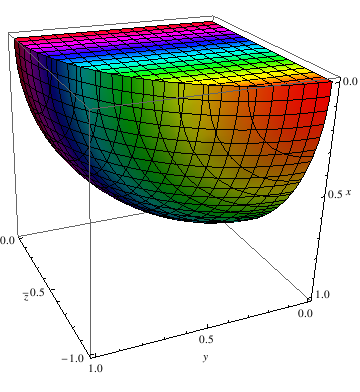
Example 1:
The paraboloid example shows that any function with three variables can be visually represented using the Plot3D function. Also, the ColorFunction option allows you to easily see the changes of the function.
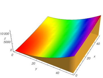 |
Plot3D[4*x^2 + y^2, {x, 0, 50}, {y, 0, 50},
Axes -> True, AxesLabel -> {y, x, z}, Boxed -> False, LabelStyle -> Italic, Mesh -> False, Filling -> Bottom, FillingStyle -> Opacity[.8], ColorFunction -> Hue, AspectRatio -> Automatic] |
Example 2:
The VectorPlot3D function is used to plot vector fields. Vector fields are used to represent equations that model many physical quantities such as the flow of liquid, strength of a force, and velocity of an object.
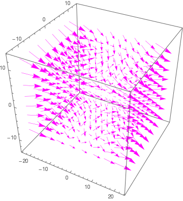 |
VectorPlot3D[{2*x^2, 3*y^2, -4*z^2}, {x, -20, 20}, {y, -10,
10}, {z, -10, 10}, BoxRatios -> {1, 1, 1}, VectorStyle -> Magenta] |
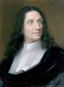
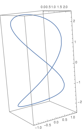
\( \mbox{viviani}[a](t) = a (1+\cos t , \sin t, 2\sin (t/2)) \qquad (-2\pi \le t \le 2\pi ) \)
To plot the viviani curve, we first define its equation and then plot it
ParametricPlot3D[viviani[1.2][t], {t, 0, 13}, PlotStyle -> Thick]
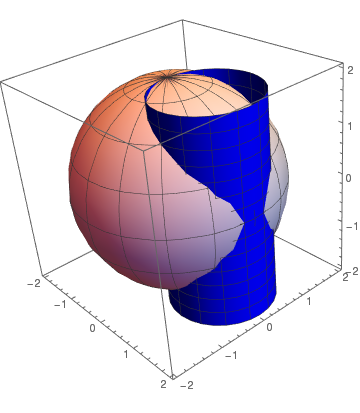
b = ParametricPlot3D[{2*Cos[t]*Cos[u], 2*Sin[t]*Cos[u], 2*Sin[u]}, {t, 0, 2*Pi}, {u, -Pi, Pi}, PlotStyle -> LightRed]
Show[b, a]
 |
 |
 |
| Vincenzo Viviani | Intersection of a cylinder with sphere | Viviani curve |
 |
 |
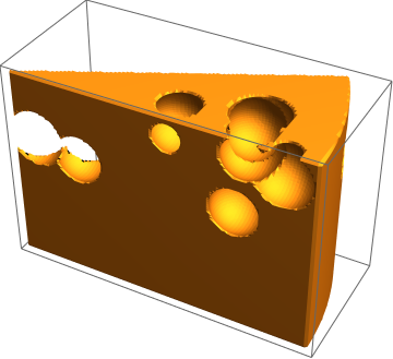
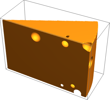
Now we randomly cut out some balls, using the RandomPoint function, to obtain a piece of cheese. This code takes a while to generate an output due to the randomness. However, each time you run the code, a new figre will appear. The following code creates a random number of balls of radius 0.65 within the three dimensional region.
 |
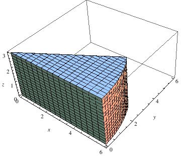
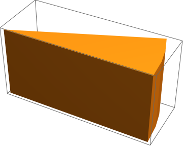
RegionPlot3D[
Fold[RegionDifference, ImplicitRegion[ x^2 + y^2 <= 6^2 && 0 < z < 4 && 0 < y <= x Sin[Pi/6], {x, y, z}], Ball[#, 0.65] & /@ RandomPoint[ ImplicitRegion[ x^2 + y^2 <= 6^2 && 0 < z < 4 && 0 < y <= x Sin[Pi/6], {x, y, z}], 10]], PlotPoints -> 100] |
The following code creates a random number of balls of radius 0.35 within the three dimensional region.
 |
RegionPlot3D[
Fold[RegionDifference, ImplicitRegion[
x^2 + y^2 <= 6^2 && 0 <= z <= 4 && 0 <= y <= x Sin[Pi/6], {x, y, z}], Ball[#, 0.35] & /@ RandomPoint[ImplicitRegion[x^2 + y^2 <= 6^2 && 0 < z < 4 && 0 < y <= x Sin[Pi/6], {x, y, z}], 10]], PlotPoints -> 100] |
The following code show more examples of plotting three dimensional regions. You may want to move the figure around to see the entire shape!
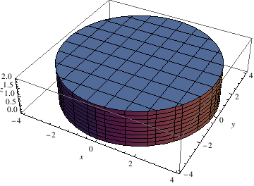 |
RegionPlot3D[x^2 + y^2 <= 16, {x, -4, 4}, {y, -4, 4}, {z, 0, 2},
BoxRatios -> Automatic, AxesLabel -> Automatic, PlotStyle -> Gray, Mesh -> 8] |
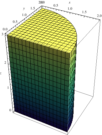 |
RegionPlot3D[x^2 + y^2 <= 4, {x, 0, 2}, {y, 0, 2}, {z, 0, 3},
BoxRatios -> Automatic, AxesLabel -> Automatic, ColorFunction -> "BlueGreenYellow"] |
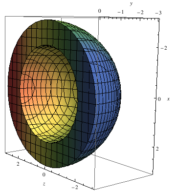 |
RegionPlot3D[
x^2 + y^2 + z^2 <= 9 && x^2 + y^2 + z^2 >= 4,
{x, -3, 3}, {y, -3, 0}, {z, -3, 3}, BoxRatios -> Automatic, AxesLabel -> Automatic, ColorFunction -> "DarkRainbow", MeshShading -> Automatic] |
 |
RegionPlot3D[x^2 + y^2 + z^2 <= 1,
{x, 0, 1}, {y, 0, 1}, {z, -1, 0}, BoxRatios -> Automatic, AxesLabel -> Automatic, ColorFunction -> Hue, MeshShading -> Automatic] |
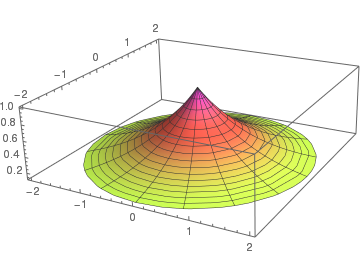
Example 5: Logarithmic functions are used to represent real world situations like population growth, decay of a substance, and financial interest rates. Most times these functions are shown in 2 dimensional spaces, but can still be represented in 3D.
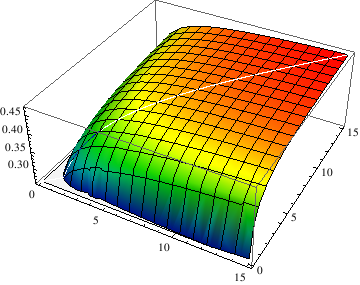 |
G[x_, y_] :=
(Log[ Min[1, (1 + x)/(1 + y)]* Min[1, (1 + y)/(1 + x)]])/(Log[(Min[x/y, y/x])^2]) Plot3D[G[x, y], {x, 0.1, 15}, {y, 0.1, 15}, ColorFunction -> Function[{x, y, z}, Hue[0.65*(1 - z)]]] |
Example 6:
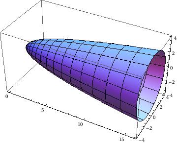
Now we plot surface of revolution with respect to x-axis.
Using the RevolutionPlot3D function, you can create a simple 2D function into a cool 3D shape:
RevolutionPlot3D[{t^2, t}, {t, 0, 4}, {\[Theta], 0, 2 Pi}, RevolutionAxis -> "X"]
 |
 |
| Revolution of parabola | Revolution of sine |
Now we plot a fancy ambrella:
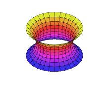
Example 7: A catenoid is a type of surface, arising by rotating a catenary curve about an axis. It is a minimal surface, meaning that it occupies the least area when bounded by a closed space. It was formally described in 1744 by the mathematician Leonhard Euler. The catenoid may be defined by the following parametric equations:
 |
 |
 |
 |
| A helicoid minimal surface formed by a soap film on a helical frame | A catenoid | A catenoid obtained from the rotation of a catenary | Deformation of a helicoid into a catenoid |
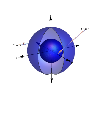
Example 8:
a = SphericalPlot3D[{1}, {\[Theta], 0, 2 Pi}, {\[Phi], 0, 4 Pi/2},
PlotStyle -> Directive[Blue, Opacity[0.5], Specularity[White, 20]],
Mesh -> None, PlotPoints -> 450];
b = SphericalPlot3D[{2}, {\[Theta], 0, Pi}, {\[Phi], 0, 5 Pi/3},
PlotStyle -> Directive[Blue, Opacity[0.5], Specularity[White, 20]],
Mesh -> {{0}, {0}, {0}}, PlotPoints -> 50];
c = Graphics3D[Arrow[Tube[{{2, 2, 2}, {1, 0, 0}}, .03]]];
d = Graphics3D[Arrow[Tube[{{0, -3, 1}, {0, -2, 1}}, .03]]];
e = Graphics3D[Arrow[{{0, 0, 0}, {3, 0, 0}}]];
f = Graphics3D[Arrow[{{0, 0, 0}, {0, -3, 0}}]];
g = Graphics3D[Arrow[{{0, 0, 0}, {0, 0, 3}}]];
h = Graphics3D[Arrow[{{0, 0, 0}, {-3, 0, 0}}]];
i = Graphics3D[Arrow[{{0, 0, 0}, {0, 3, 0}}]];
j = Graphics3D[Arrow[{{0, 0, 0}, {0, 0, -3}}]];
k = Graphics3D[Text[P == 1, {2, 2, 2}]];
l = Graphics3D[Text[P == 2, {0, -3, 1}]];
m = Graphics3D[Text[x, {0, -3.1, 0}]];
n = Graphics3D[Text[y, {3.1, 0, 0}]];
o = Graphics3D[Text[z, {0, 0, 3}]];
az = Show[a, b, c, d, e, f, g, h, i, j, k, l, m, n, o,
PlotRange -> {{-3, 3}, {-3, 3}, {-3, 3}},
Axes -> {False, False, False}, Boxed -> False]
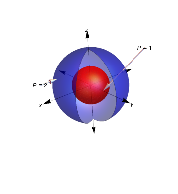
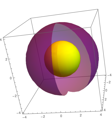
We can plot sphere with different colors.
b = SphericalPlot3D[{2}, {\[Theta], 0, Pi}, {\[Phi], 0, 5 Pi/3},
PlotStyle -> Directive[Blue, Opacity[0.5], Specularity[White, 20]],
Mesh -> {{0}, {0}, {0}}, PlotPoints -> 50];
c = Graphics3D[Arrow[Tube[{{2, 2, 2}, {1, 0, 0}}, .03]]];
d = Graphics3D[Arrow[Tube[{{0, -3, 1}, {0, -2, 1}}, .03]]];
e = Graphics3D[Arrow[{{0, 0, 0}, {3, 0, 0}}]];
f = Graphics3D[Arrow[{{0, 0, 0}, {0, -3, 0}}]];
g = Graphics3D[Arrow[{{0, 0, 0}, {0, 0, 3}}]];
h = Graphics3D[Arrow[{{0, 0, 0}, {-3, 0, 0}}]];
i = Graphics3D[Arrow[{{0, 0, 0}, {0, 3, 0}}]];
j = Graphics3D[Arrow[{{0, 0, 0}, {0, 0, -3}}]];
k = Graphics3D[Text[P == 1, {2, 2, 2}]];
l = Graphics3D[Text[P == 2, {0, -3, 1}]];
m = Graphics3D[Text[x, {0, -3.1, 0}]];
n = Graphics3D[Text[y, {3.1, 0, 0}]];
o = Graphics3D[Text[z, {0, 0, 3}]];
az = Show[a, b, c, d, e, f, g, h, i, j, k, l, m, n, o,
PlotRange -> {{-3, 3}, {-3, 3}, {-3, 3}},
Axes -> {False, False, False}, Boxed -> False]
Two spheres
Two spheres with different colors
c = SphericalPlot3D[4, {\[Theta], 0, \[Pi]}, {\[Phi], 1, 2 \[Pi]}]
d = SphericalPlot3D[2, {\[Theta], 0, Pi}, {\[Phi], 0, 2 Pi}]
Show[c, d]
d = SphericalPlot3D[2, {\[Theta], 0, Pi}, {\[Phi], 0, 2 Pi}, Mesh -> None, PlotStyle -> Yellow];
Show[c, d]
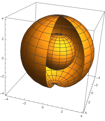 |
 |
| Two spheres | Two spheres with different colors |
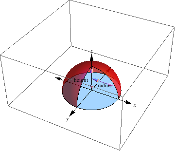
The following script can be used to display arrows and text to specifically illustrate dimensions.
a = Graphics3D[Arrow[Tube[{{0, 0, 1}, {0, 0, 2}}, .025]]];
c = Graphics3D[Arrow[Tube[{{0, 0, 1}, {0, 0, 0}}, .025]]];
o = Graphics3D[Text[height, {-0.5, -0.5, 1}]];
p = Graphics3D[Arrow[Tube[{{1, 0, 1}, {0, 0, 1}}, .025]]];
q = Graphics3D[Arrow[Tube[{{1, 0, 1}, {1.75, 0, 1}}, .025]]];
r = Graphics3D[Text[radius, {1, 0, 0.8}]];
d = Graphics3D[Cylinder[{{0, 0, 0}, {0, 0, .0001}}, 2]];
b = SphericalPlot3D[{2}, {\[Theta], 0, Pi}, {\[Phi], 0, 3 Pi/2},
PlotStyle -> Directive[Red, Opacity[0.7], Specularity[White, 20]],
Mesh -> {{0}, {0}, {0}}, PlotPoints -> 40];
g = Graphics3D[Arrow[{{0, 0, 0}, {0, 0, 3}}]];
h = Graphics3D[Arrow[{{0, 0, 0}, {0, -3, 0}}]];
i = Graphics3D[Arrow[{{0, 0, 0}, {3, 0, 0}}]];
j = Graphics3D[Text[z, {0, 0, 3.2}]];
k = Graphics3D[Text[x, {3.2, 0, 0}]];
l = Graphics3D[Text[y, {0, -3.2, 0}]];
m = Graphics3D[Arrow[{{0, 0, 0}, {-3, 0, 0}}]];
n = Graphics3D[Arrow[{{0, 0, 0}, {0, 3, 0}}]];
b = Show[a, b, c, d, g, h, i, j, k, l, m, n, o, p, q, r,
PlotRange -> {{-4, 4}, {-4, 4}, {0, 4}}]
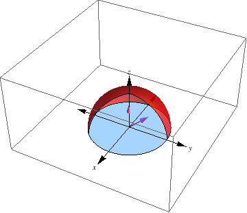
a = Graphics3D[Arrow[Tube[{{0, 0, 0}, {0, 0, Sqrt[2]}}, .025]]];
c = Graphics3D[Arrow[Tube[{{0, 0, 0}, {1, 0, 1}}, .025]]];
d = Graphics3D[Cylinder[{{0, 0, 0}, {0, 0, .0001}}, 2]];
b = SphericalPlot3D[{2}, {\[Theta], 0, Pi}, {\[Phi], 0, 5 Pi/4},
PlotStyle -> Directive[Red, Opacity[0.7], Specularity[White, 20]],
Mesh -> {{0}, {0}, {0}}, PlotPoints -> 40];
g = Graphics3D[Arrow[{{0, 0, 0}, {0, 0, 3}}]];
h = Graphics3D[Arrow[{{0, 0, 0}, {0, -3, 0}}]];
i = Graphics3D[Arrow[{{0, 0, 0}, {3, 0, 0}}]];
j = Graphics3D[Text[z, {0, 0, 3.2}]];
k = Graphics3D[Text[y, {3.2, 0, 0}]];
l = Graphics3D[Text[x, {0, -3.2, 0}]];
m = Graphics3D[Arrow[{{0, 0, 0}, {-3, 0, 0}}]];
n = Graphics3D[Arrow[{{0, 0, 0}, {0, 3, 0}}]];
b = Show[a, b, c, d, g, h, i, j, k, l, m, n,
PlotRange -> {{-4, 4}, {-4, 4}, {0, 4}}]
RegionPlot3D[
x^2 + y^2 <= 6^2 && 0 < z < 4 && 0 < y <= .1 x Sin[Pi/6], {x, 0,
6}, {y, 0, Sin[Pi/6]}, {z, 0, 4}]
a = SphericalPlot3D[4, {\[Theta], 0, \[Pi]/2}, {\[Phi], 1, 2 \[Pi]}]
b = SphericalPlot3D[4, {\[Theta], .8, \[Pi]/2}, {\[Phi], 0, 2 \[Pi]}]
Show[a, b]
One can put a box inside a sphere:
e = SphericalPlot3D[4, {\[Theta], 0, \[Pi]/2}, {\[Phi], 3, 2 \[Pi]}]
f = Graphics3D[Cuboid[{-2, -1, 2}]]
Show[e, f]
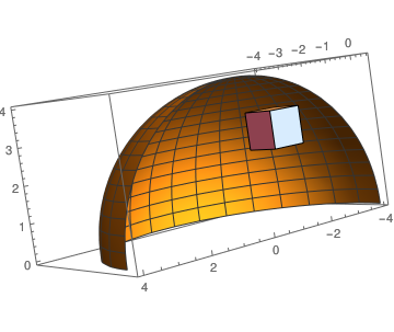 |
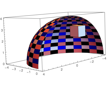 |
| Spherical shell with a box | Meshed spherical shell with a box |
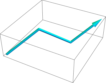
Example 9: Arrow plots can be used to show the direction of a line by adding arrows to the functions. A typical arrow plot:
Arrow[Tube[ Table[{Cos[phi], Sin[phi], .2 phi}, {phi, 0, 10, 0.1}]]] // Graphics3D
or using colors
 |
 |
 |
| Typical arrow | Colored arrow | Colored line arrow |
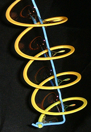
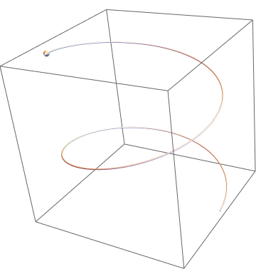
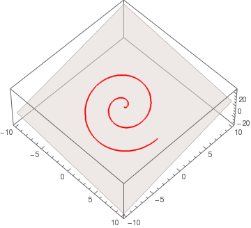
{x[t], y[t]} = {t Cos[2 t], t Sin[2 t]} and a plane:
3 (x + 1) - 2 (y - 2) + (z - 3) = 0. The spiral must be centered
at {-1, 2, 3}. Since the given plane is already in a convenient
form, we can easily extract the center point and the normal of the plane to
use with RotationTransform[] and InfinitePlane[]. Thus,
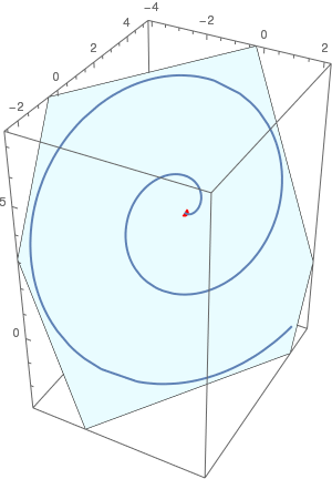 |
With[{pt = {-1, 2, 3}, nrm = {3, -2, 1}},
Show[ParametricPlot3D[ pt + RotationTransform[{{0, 0, 1}, nrm}][ {t Cos[2 t], t Sin[2 t], 0}] // Evaluate, {t, 0, 2 π}], Graphics3D[{{Red, AbsolutePointSize[8], Point[pt]}, {LightBlue, InfinitePlane[pt, Rest[Orthogonalize[{nrm, {1, 0, 0}, {0, 1, 0}}]]]}}], Lighting -> "Neutral"]] |
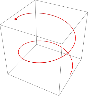
Or the same plot can be obtained with a sequence of commands. First, we define the point
p = {-1, 2, 3}; point = ListPointPlot3D[{p}, PlotStyle -> {Blue, PointSize[Large]}]
the plane
eqPlane = 3 (x + 1) - 2 (y - 2) + (z - 3) == 0;
f[x_, y_] := z /. First @ Solve[eqPlane, z]
f[x, y]
plane = ParametricPlot3D[{x, y, f[x, y]}, {x, -10, 10}, {y, -10, 10}, Mesh -> None, BoxRatios -> 1
{a[t_], b[t_], c[t_]} := {t Cos[2 t], t Sin[2 t], f[a[t], b[t]]}
and the origin of the spirals0 = {a[0], b[0], c[0]}
Plot of the spiral moved to the point p:
spiral = ParametricPlot3D[{a[t], b[t], c[t]} - s0 + p, {t, 0, 2 π}, PlotStyle -> Red, BoxRatios -> 1]
view = Coefficient[Simplify[First@eqPlane], #] & /@ {x, y, z}
Show[spiral, plane, point, ViewPoint -> view]
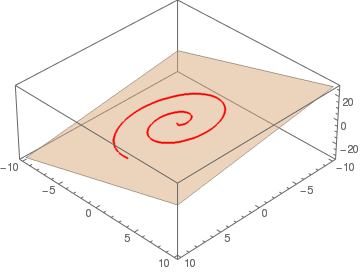
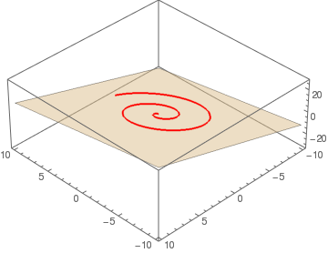
{x[t_], y[t_]} = {t Cos[2 t], t Sin[2 t]};
p = ({x, y, z} /. First@Solve[(x + 1) - 2 (y - 2) + (z - 3) == 0, z])
q = p /. {x -> x[t], y -> y[t]};
Show[Plot3D[Evaluate[p[[3]]], {x, -10, 10}, {y, -10, 10},
Mesh -> None, PlotStyle -> {LightBlue, Opacity[0.5]}, ViewPoint -> {5, 5, 5}],
ParametricPlot3D[Evaluate[q], {t, 0, 2 Pi}, PlotStyle -> Red]]
| View point (5,5,5) | View point (-5,5,5) | View point (5,-5,d105) |
|---|---|---|
|
|
 |
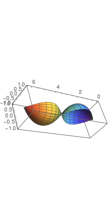
Another beautiful command SliceContourPlot3D generates a contour plot of a function over the slice surface as a function of x, y and z. For example, we plot the contours over the surface x³ + 2 y² - 3 z² = 0.
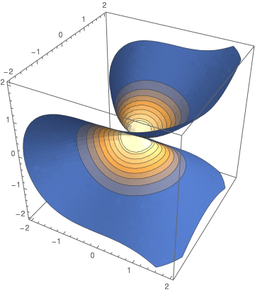 |
SliceContourPlot3D[Exp[-(x^2 + y^2 + z^2)], x^3 + 2 y^2 - 3 z^2 == 0, {x,-2,2}, {y,-2,2}, {z,-2,2}]
|
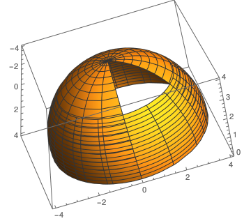
Ambrella:
RevolutionPlot3D[Exp[-x], {x, 0, 2}]
|
|
RevolutionPlot3D[Exp[-x], {x, 0, 2}]
|
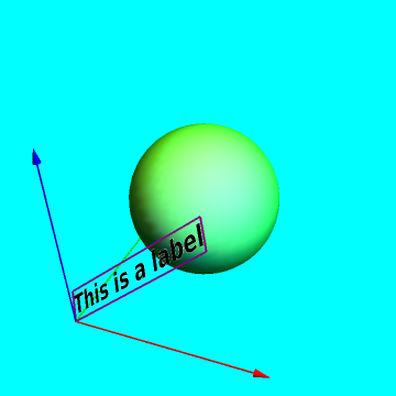
The function label3D takes an arbitrary expression and displays it as a textured 3D rectangle with transparent background. The expression is converted to an image without being evaluated. By default, regions matching the color at the corner of the image are made transparent. Alternatively, you can explicitly specify which color to make transparent by adding the option "TransparentColor" → White to label3D (instead of White, the color can be anything you like).
Module[{ra, width, height, r},
ra = Rasterize[
Style[HoldForm[s], FilterRules[{opts}, Options[Style]], Magnification -> 10],
Evaluate@Apply[Sequence, FilterRules[{opts}, Options[Rasterize]]], "Image" ];
{width, height} = ImageDimensions[ra];
r = SetAlphaChannel[ra, With[
{
color = Apply[List, ColorConvert[
"TransparentColor" /. {opts} /. {"TransparentColor" ->
Apply[RGBColor, ImageData[ra][[2, 2]]]}, "RGB"] ]
}, Binarize[ra, (Norm[# - color] > .005)&]]
];
Translate[(* // to make lefthand corner pos *)
Rotate[(* // around z axis *)
Rotate[ (* // around y axis *)
Rotate[(* // tilt around x axis *)
Scale[ (*// to make width equal |xVec| *)
{EdgeForm[FrameStyle /. {opts} /. FrameStyle -> None],
Texture[ImageData@r],
(* // Texture fills polygon initially in the xz plane *)
Polygon[{{0, 0, 0}, {width, 0, 0}, {width, 0, height}, {0, 0, height}},
VertexTextureCoordinates -> {{0, 0}, {1, 0}, {1, 1}, {0, 1}}]},
Norm[xVec]/width, {0, 0, 0} ],
tiltAngle, {1, 0, 0}],(* // x rotation *)
Arg[Chop@N[Norm[xVec[[1 ;; 2]]] + I xVec[[3]]]], {0, -1, 0}], (* // y rotation *)
Arg[Chop@N[xVec[[1]] + I xVec[[2]]]], {0, 0, 1} ], (* // z rotation *)
pos]
];
SetAttributes[label3D, HoldFirst]
|
To write labels on the graph:
With[{position = {0, 0, 0}, direction = {1.5, 0, 1.3},
tiltAngle = -.8}, Graphics3D[{{Green, Specularity[2], Sphere[{1, 1, 1}, .7]}, Map[{Apply[RGBColor, #], Arrow[Tube[{{0, 0, 0}, #}]]} &, 2 IdentityMatrix[3]], {Glow[White], label3D["This is a label", position, direction, tiltAngle, FontColor -> Black, FontSize -> 18, FontFamily -> "Helvetica", FontWeight -> Bold, Magnification -> 4, FrameStyle -> Directive[Purple, Thick]]}}, Boxed -> False, SphericalRegion -> True, Background -> Cyan]] |
- Visualization and Graphics by John Boccio, Wolfram Mathematica Tutorial Collection.
Return to Mathematica page
Return to the main page (APMA0340)
Return to the Part 1 Matrix Algebra
Return to the Part 2 Linear Systems of Ordinary Differential Equations
Return to the Part 3 Non-linear Systems of Ordinary Differential Equations
Return to the Part 4 Numerical Methods
Return to the Part 5 Fourier Series
Return to the Part 6 Partial Differential Equations
Return to the Part 7 Special Functions