Preface


In 1747, d'Alembert derived the first partial differential equation (PDE for short) in the history of mathematics, namely the wave equation. This section provides an introduction to one-dimensional wave equations and corresponding initial value problems.

Return to computing page for the first course APMA0330
Return to computing page for the second course APMA0340
Return to Mathematica tutorial for the first course APMA0330
Return to Mathematica tutorial for the second course APMA0340
Return to the main page for the first course APMA0330
Return to the main page for the second course APMA0340
Return to Part VI of the course APMA0340
Introduction to Linear Algebra with Mathematica

Wave Equation


Jean le Rond d'Alembert

The wave equation is a typical example of more general class of partial differential equations called hyperbolic equations. They occur in classical physics, geology, acoustics, electromagnetics, and fluid dynamics. Wave equations usually describe wave propagations in different media. 
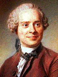
Historically, the problem of a vibrating string such as that of a musical instrument was first studied by the French mathematician, mechanical physicist, philosopher, and music theorist Jean le Rond d'Alembert. Because he was the first who found a solution of one-dimensional wave equation in 1746, the latter is usually referred to as d'Alembert's equation. Many others contributed to study of the wave equation, among first of them we mention Leonhard Euler (who discovered the wave equation in three space dimensions), Daniel Bernoulli ( the Euler–Bernoulli beam equation), and Joseph-Louis Lagrange (classical and celestial mechanics).

The wave equation for real-valued function \( u(x_1, x_2, \ldots , x_n , t) \) of n spatial variables and a time variable t is

\begin{equation} \label{EqWave.1} \frac{\partial^2 u}{\partial t^2} = c^2 \nabla^2 u , \qquad \mbox{or} \qquad \square u =0 , \end{equation}
where c is a positive constant (having dimensions of speed) and
\begin{equation} \label{EqWave.2} \nabla^2 u \equiv \Delta u = \frac{\partial^2 u}{\partial x_1^2} + \frac{\partial^2 u}{\partial x_2^2} + \cdots + \frac{\partial^2 u}{\partial x_n^2} \qquad\mbox{and} \qquad \square u \equiv \square_c u = \frac{\partial^2 u}{\partial t^2} - c^2 \Delta u . \end{equation}
The differential operator □ is called the d'Alembertian and △ is the Laplacian.

Suppose we have a medium whose displacement may be described by a scalar function u(x,t), where \( {\bf x} \in \mathbb{R}^n , \quad t\in\mathbb{R} . \) Suppose that the system is conservative and it has the Lagrangian \( {\cal L} = \mbox{K} - \Pi , \) where the kinetic energy K and potential energy Π of the medium are

\[ \mbox{K} \left( u_t \right) = \frac{1}{2} \int \rho\,u_t\,{\text d}{\bf x} , \qquad \Pi \left( u \right) = \frac{1}{2} \int k \left\vert \nabla u \right\vert^2 {\text d}{\bf x} . \]
Here ρ(x) is a mass-density and k(x) is a stiffness, both assumed positive, and \( u_t = \partial u/\partial t . \) The corresponding action becomes
\[ S \left( u \right) = \int {\text d}t \, {\cal L} \left( u, u_t \right) = \int {\text d}t \int {\text d}{\bf x} \,\frac{1}{2} \left\{ \rho\,u_t^2 - k\left\vert \nabla u \right\vert^2 \right\} . \]
Note that the kinetic and potential energies and the Lagrangian are functions of the spacial field and velocity at each fixed time, whereas the action is a functional of the space-time field u(x, t), obtained by integrating the Lagrangian with respect to time.

The Euler--Lagrange equation is satisfied by a stationary point (which is a function u(x, t)) of this action becomes

\[ \rho\, u_{tt} - \nabla \cdot \left( k\,\nabla u \right) =0 . \]
If ρ and k are constants, then we get the wave equation
\[ \square_c u \equiv u_{tt} - c^2 \Delta u =0 \qquad\mbox{or}\qquad \frac{\partial^2 u}{\partial t^2} - c^2 \nabla^2 u =0 . \]
The action functional for the wave equation is not positive definite. Therefore, we cannot expect a solution of the wave equation to be a minimizer of the action, in general, only a critical point.   ■

We derive the wave equation in one space dimension that models the transverse vibrations of an elastic string. If such string is placed horizontally between end points x=0 and x=ℓ, it can freely vibrate within a vertical plane. Generally speaking it is not true; however, if displacements u(x,t) are small, we can assume that spring motion occur only within a plane perpendicular to its equilibrium horizontal position.


Perhaps the easiest case is observed with the investigation of mechanical vibrations. Suppose that an elastic string of length ℓ is tightly stretched between two supports at the same horizontal level, which we identify with x-axis. Then its end points may be taken as x=0 and x=ℓ. The elastic string may be thought of as a guitar or violin string, a guy wire, or possibly an electric power line. The positions of points on the string can be described by the displacement, which we denote by u(x,t), from the equilibrium horizontal position. If damping effects, such as air resistance, are neglected, and if the magnitude of the motion is not too large, then the displacement function satisfies the partial differential equation (called one dimensional wave equation)

\[ \square_c u =0 \qquad\mbox{or} \qquad u_{tt} = c^2 u_{xx} \]
in the domain 0 < x < ℓ    0 < t < ∞. The constant coefficient c² is given by
\[ c^2 = T/\rho , \]
where T is the tension (force) in the string, and ρ is the mass per unit length of the string material (density). To describe the motion of the string completely, we need to impose some auxiliary conditions. Of these, we need to specify the initial displacement and its initial velocity
\[ u(x,0) = d(x), \qquad \dot{u} (x,0) \equiv \left. \frac{\partial u}{\partial t} \right\vert_{t=0} = v(x) , \]
where d and v are known functions. If we consider a ideal (and not realistic) case that the string has an infinite length, we arrive at so called the initial value problem:
\[ u_{tt} = c^2 u_{xx}, \qquad u(x,0) = d(x), \qquad \dot{u} (x,0) = v(x) , \qquad -\infty < x < \infty . \]
This problem was first solved by Jean d'Alembert, which is presented below.

The one dimensional d'Alembertian operator can be recomposed into the product of the first order differential operators:

\[ \square_c \equiv \frac{\partial^2 }{\partial t^2} - c^2 \frac{\partial^2 }{\partial x^2} = \left( \frac{\partial}{\partial t} - c\,\frac{\partial}{\partial x} \right) \left( \frac{\partial}{\partial t} + c\,\frac{\partial}{\partial x} \right) \]
This allows one to reduce the second order partial differential equation utt - c²uxx = 0 to two first order equations
\[ \frac{\partial v}{\partial t} - c\,\frac{\partial v}{\partial x} =0 \qquad\mbox{and}\qquad \frac{\partial v}{\partial t} + c\,\frac{\partial v}{\partial x} =0. \]
By introducing a new variable ξ = x ±ct, each of the above equations is reduced to a simple ordinary differential equation
\[ \frac{{\text d} v}{{\text d} \xi} = \frac{\partial v}{\partial x}\,\frac{\partial x}{\partial \xi} + \frac{\partial v}{\partial t}\,\frac{\partial t}{\partial \xi} = \frac{\partial v}{\partial x} \pm \frac{1}{c}\,\frac{\partial v}{\partial t} =0, \]
which can be integrated directly. This leads to the conclusion that a solution of the wave equation utt - c²uxx = 0 is the sum
\[ u(x,t) = f(x+ct) + g(x-ct) \]
of two functions f(ξ) and g(ξ) of one variable. This formula represents a superposition of two waves, one traveling to the right and another traveling to the left, each with velocity x. However, in practice, traveling waves are excited by the initial disturbance
\[ u(x,0) = d(x) \qquad \mbox{and}\qquad \left. \frac{\partial u}{\partial t} \right\vert_{t=0} = v(x) , \]
where d(x) is the initial displacement (initial configuration) and v(x) is the initial velocity of the string. Upon substituting the general solution into the initial condition, we get two equations
\[ \begin{split} d(x) &= f(x) + g(x) , \\ v(x) &= c\, f' (x) - c\, g' (x) . \end{split} \]
Integrating the latter, we obtain
\[ \int_0^x v(\xi )\,{text d}\xi = c\,f(x) - c\,g(x) . \]
This enables us to express the general solution in terms of the initial displacement and the initial velocity (called the d'Alembert's formula)
\[ u(x,t) = \frac{d(x+ct) + d(x-ct)}{2} + \frac{1}{2c} \,\int_{x-ct}^{x+ct} v(\xi )\,{\text d}\xi . \]
   ■

Energy method. Suppose a twice differentiable function u(x,t) is a solution of the initial value problem

\[ \begin{cases} u_{tt} &= c^2 \Delta u, \qquad {\bf x} \in \mathbb{R}^n , \quad 0 < t , \\ u({\bf x}, 0) &= d({\bf x}) , \qquad u_t ({\bf x},0) = v({\bf x}) , \end{cases} \]
where the given continuous functions d(x) and v(x) are assumed to be zero outside some disk. We define the energy function as a function of time variable t:
\[ E(t) = \frac{1}{2} \int_{\mathbb{R}^n} \left( u_t^2 + c^2 \left\vert \nabla u \right\vert^2 \right) {\text d} {\bf x} . \]
The derivative of the energy function is
\begin{align*} \frac{{\text d} E}{{\text d}t} &= \frac{{\text d}}{{\text d}t} \left[ \frac{1}{2} \int_{\mathbb{R}^n} \left( u_t^2 + c^2 \left\vert \nabla u \right\vert^2 \right) {\text d} {\bf x} \right] = \int_{\mathbb{R}^n} \left( u_t u_{tt} + c^2 \sum_{i=1}^n u_{x_i} u_{x_i t} \right) {\text d} {\bf x} \\ &= \int_{\mathbb{R}^n} u_t u_{tt} \, {\text d} {\bf x} + c^2 \left[ \sum_{i=1}^n u_{x_i} u_t \right]_{\partial \mathbb{R}^n} - c^2 \int_{\mathbb{R}^n} \sum_{i=1}^n u_{x_i x_i} u_t \,{\text d} {\bf x} \\ &= \int_{\mathbb{R}^n} u_t \left( u_{tt} - c^2 \Delta u \right) {\text d} {\bf x} = 0 . \end{align*}
Hence, the nergy function E(t) is a constant, so E(t) = E(0).

In particular, if u1 and u2 are two solutions of the initial value problem for the wave equation, then v = u1 - u2 has homogeneous initial conditions, and so E(t) = E(0) = 0. Since the nonnegative energy function is a constant, it implies that v = 0. So the solution of such Cauchy problem is unique.    ▣

Example: Dirichlet boundary conditions. Let us consider the vibrations of an infinitely long string (0 < x < ∞) that is fixed at one end. We first assume that the boundary condition at left end x = 0 are of first type (Dirichlet):

\[ \left\{ \begin{array}{ll} \ddot{u} = c^2 u_{xx} , & 0 < x < \infty ,\quad 0<t<t^{\ast} <\infty ; \\ u(0,t) =0, & 0 < t< t^{\ast} < \infty ; \\ u(x,0) = d(x) , \quad \dot{u} (x,0) = v(x) ,\quad & 0<x<\infty . \end{array} \right. \]
As usual, the dot indicates derivative with respect to time variable: \( \dot{u} = \partial u/\partial t \) and \( \ddot{u} = \partial^2 u/\partial t^2 . \) To understand the solution, we assume temporally that input is a snakey. (A "snakey" is a slinky-like device that consists of a large concentration of small-diameter metal coils.) If an upward displaced pulse is introduced at the left end of the snakey, it will travel rightward across the snakey until it reaches the fixed end on the right side of the snakey. Upon reaching the fixed end, the single pulse will reflect and undergo inversion. That is, the upward displaced pulse will become a downward displaced pulse. Now suppose that a second upward displaced pulse is introduced into the snakey at the precise moment that the first crest undergoes its fixed end reflection. If this is done with perfect timing, a rightward moving, upward displaced pulse will meet up with a leftward moving, downward displaced pulse in the exact middle of the snakey. As the two pulses pass through each other, they will undergo destructive interference. The animation below shows several snapshots of the meeting of the two pulses at various stages in their interference.
To derive the appropriate formula, we recall that d'Alembert solution
\[ u(x,t) = \frac{1}{2} \left[ d(x-ct) + d(x+ct) \right] + \frac{1}{2c} \int_{x-ct}^{x+ct} v(s)\, {\text d} s \]
is valid only for 0 < x < ∞ since the initial displacement d(x) and the initial velocity v(x) are defined only for positive inputs. Therefore, the d'Alembert formula provides a solution to the wave equation only when x ±ct > 0. Since all ingredients (x, c, t) are positive, the expression x + ct > 0 always true. If x - ct > 0, then the d'Alembert solution is still valid. However, for negative values, it is false.

Now suppose that x - ct ≤ 0. Using the traveling wave formula \( u(x,t) = F(x-ct) + G(x+ct) , \) we try to satisfy the Dirichlet boundary condition

\[ u(x,0) = F(-ct) + G(ct) = 0 . \]
Let w = -ct, so F(w) = -G(-w) for w ≤ 0, which reveals how the function F(w) should be defined. Therefore,
\begin{align*} u(x,t) &= F(x-ct) + G(x+ct) = - G(ct-x) + G(x+ct) \\ &= \frac{1}{2} \left[ d(x+ct) - d(ct-x) \right] + \frac{1}{2c} \int_{ct-x}^{x+ct} v(s)\,{\text d} s, \end{align*}
for x - ct ≤ 0. Finally, we combine it with the d'Alembert solution to obtain
\[ u(x,t) = \begin{cases} \frac{1}{2} \left[ d(x+ct) - d(ct-x) \right] + \frac{1}{2c} \int_{ct-x}^{x+ct} v(s)\,{\text d} s, \quad x-ct \le 0, \\ \frac{1}{2} \left[ d(x+ct) + d(x-ct) \right] + \frac{1}{2c} \int_{x-ct}^{x+ct} v(s)\,{\text d} s, \quad x-ct > 0 . \end{cases} \]


We can solve the above initial value problem using sine Fourier transform. To do this, we multiply both sides of the wave equation by \( \sin (kx) \) and integrate with respect to variable x from zero to infinity. Then integration by parts leads to
\[ \frac{{\text d}^2 u^S}{{\text d}t^2} + c^2 k^2 u^S = -k\,u(0,t) \ (0< t < \infty ), \qquad u^S (k, 0) = d^S , \quad \dot{u}^S (0) = v^S . \]
Here uS, dS, and vS are sine Fourier transforms of functions u, d, and v, respectively:
\[ u^S (k,t) = ℱ_s \left[ u(x,t) \right] = \int_0^{\infty} u(x,t) \,\sin (kx)\,{\text d}x , \quad d^S (k) = ℱ_s \left[ d(x) \right] = \int_0^{\infty} d(x) \,\sin (kx)\,{\text d}x , \quad v^S (k) = ℱ_s \left[ v(x) \right] = \int_0^{\infty} v(x) \,\sin (kx)\,{\text d}x . \]
Solution uS of the above initial value problem is exactly the same as the corresponding solution for Neumann problem:
\[ u^S (k,t) = \frac{1}{ck} \left[ k\,d^C \cos (ckt) + v^C \sin (ckt) \right] . \]
Application of the inverse since Fourier transform yeilds
\[ u(x,t) = ℱ_s^{-1} \left[ u^S (k,t) \right] = \frac{2}{\pi} \int_0^{\infty} \left[ \frac{1}{c}\, d^C \cos (ckt) + v^C \,\frac{\sin (ckt)}{ck} \right] \sin (kx)\,{\text d}k . \]
Using the convolution rule, we get
\[ u(x,t) = \frac{1}{2} \int_0^{\infty} d(\xi ) \left[ \psi (x-\xi ) - \psi (x+\xi ) \right] {\text d}\xi + \frac{1}{2} \int_0^{\infty} v(\xi ) \left[ \phi (x-\xi ) - \phi (x+\xi ) \right] {\text d}\xi , \]
where
\begin{align*} \psi (x) &= \frac{2}{\pi} \int_0^{\infty} \frac{1}{c}\, \cos (ckt)\,\sin (kx)\,{\text d}k , \\ \phi (x) &= \frac{2}{\pi} \int_0^{\infty} \frac{\sin (ckt)}{ck} \,\sin (kx)\,{\text d} k . \end{align*}
Mathematica helps
Assuming[y > 0 && x > 0, Integrate[Sin[k*y]*Sin[k*x]/k, {k, 0, Infinity}]]
1/2 Log[(x + y)/Abs[x - y]]
So we have
\[ \phi (x,t) = \frac{2}{\pi} \int_0^{\infty} \frac{\sin (ckt)}{ck} \,\sin (kx)\,{\text d} k = \frac{1}{c\pi} \,\ln \frac{ct+x}{|ct-x|} . \]
Function ψ is the derivative (in weak sense because the integral does not converge in regular sense) with respect to time variable of function ϕ:
\[ \psi (x,t) = \frac{\partial}{\partial t}\, \phi (x,t) = \frac{\partial}{\partial t}\, \frac{1}{c\pi} \,\ln \frac{ct+x}{|ct-x|} . \]
We determine the expression for function ψ from the limit:
\begin{align*} \psi (x,t) &= \lim_{\epsilon \to 0} \frac{2}{c\pi} \int_0^{\infty} \cos (ckt)\,\sin (kx)\,e^{-\epsilon k} {\text d}k = \lim_{\epsilon \to 0} \frac{2x \left( \epsilon^2 - c^2 t^2 + x^2 \right)}{c\pi \left( \epsilon^2 + (x-ct)^2 \right)\left( \epsilon^2 + (x-ct)^2 \right)} \\ &= \frac{2x}{c\pi \left( x- ct \right)\left( x+ ct \right)} \end{align*}
Assuming[c > 0 && t > 0 && eps > 0 && x > 0, 2/Pi/c*Integrate[Exp[-eps*k]*Cos[c*k*t]*Sin[k*x], {k, 0, Infinity}]]
(2 x (eps^2 - c^2 t^2 + x^2))/(c \[Pi] (eps^2 + (-c t + x)^2) (eps^2 + (c t + x)^2))
Similar for ϕ:
Assuming[c > 0 && t > 0 && eps > 0 && x > 0, 2/Pi/c*Integrate[ Exp[-eps*k]*Sin[c*k*t]*Sin[k*x]/k, {k, 0, Infinity}]]
Log[(eps^2 + (c t + x)^2)/(eps^2 + (-c t + x)^2)]/(2 c \[Pi])
\[ \phi (x,t) = \lim_{\epsilon \to 0} \frac{2}{c\pi} \int_0^{\infty} \cos (ckt)\,\sin (kx)\,e^{-\epsilon k} \frac{{\text d}k}{k} = \frac{1}{2c\pi} \, \ln \frac{\left( x+ct \right)^2}{\left( x-ct \right)^2} . \]


Example: Neumann boundary conditions. Now we consider the same problem, but with Neumann boundary conditions
\[ \left\{ \begin{array}{ll} \ddot{u} = c^2 u_{xx} , & 0 < x < \infty ,\quad 0<t<t^{\ast} <\infty ; \\ u_x (0,t) =0, & 0 < t< t^{\ast} < \infty ; \\ u(x,0) = d(x) , \quad \dot{u} (x,0) = v(x) ,\quad & 0<x<\infty . \end{array} \right. \]
Using a similar strategy, we derive its solution to be
\[ u(x,t) = \begin{cases} \frac{1}{2} \left[ d(x+ct) + d(ct-x) \right] + \frac{1}{2c} \int_0^{ct-x} v(s)\,{\text d} s + \frac{1}{2c} \int_0^{x+ct} v(s)\,{\text d} s , \quad x-ct \le 0, \\ \frac{1}{2} \left[ d(x+ct) + d(x-ct) \right] + \frac{1}{2c} \int_{x-ct}^{x+ct} v(s)\,{\text d} s, \quad x-ct > 0 . \end{cases} \]


Now we solve the same problem with the aid of cosine Fourier transform. Its application yilds
\[ \frac{{\text d}^2 u^C}{{\text d}t^2} + c^2 k^2 u^C = u_x (0,t) \ (0< t < \infty ), \qquad u^S (k, 0) = d^C , \quad \dot{u}^C (0) = v^D . \]
Here uC, dC, and vC are cosine Fourier transforms of functions u, d, and v, respectively:
\[ u^C (k,t) = ℱ_c \left[ u(x,t) \right] = \int_0^{\infty} u(x,t) \,\cos (kx)\,{\text d}x , \quad d^C (k) = ℱ_c \left[ d(x) \right] = \int_0^{\infty} d(x) \,\cos (kx)\,{\text d}x , \quad v^S (k) = ℱ_c \left[ v(x) \right] = \int_0^{\infty} v(x) \,\cos (kx)\,{\text d}x . \]
Assuming[ k > 0, DSolve[{u''[t] == -k^2 *u[t], u[0] == a, u'[0] == b}, u[t], t]]
{{u[t] -> (a k Cos[k t] + b Sin[k t])/k}}
The above initial value problem has a unique solution:
\[ u^C (k,t) = \frac{1}{ck} \left[ k\,d^C \cos (ckt) + v^C \sin (ckt) \right] . \]
Taking inverse cosine Fourier transform, we obtain the solution
\[ u(x,t) = ℱ_c{-1} \left[ u^C (k,t) \right] = \frac{2}{\pi} \int_0^{\infty} \left[ \frac{1}{c}\, d^C \cos (ckt) + v^C \,\frac{\sin (ckt)}{ck} \right] \cos (kx)\,{\text d}k . \]
Using the convolution rule, we get
\[ u(x,t) = \frac{1}{2} \int_0^{\infty} d(\xi ) \left[ \psi (x-\xi ) + \psi (x+\xi ) \right] {\text d}\xi + \frac{1}{2} \int_0^{\infty} v(\xi ) \left[ \phi (x-\xi ) + \phi (x+\xi ) \right] {\text d}\xi , \]
where
\begin{align*} \psi (x) &= \frac{1}{\pi} \int_0^{\infty} \frac{1}{c}\, \cos (ckt)\,\cos (kx)\,{\text d}k , \\ \phi (x) &= \frac{2}{\pi} \int_0^{\infty} \frac{\sin (ckt)}{ck} \,\cos (kx)\,{\text d} k . \end{align*}
Although the inetgral for ϕ does not exist in ordinary sense, it is a week derivative of ψ, so we find first its value:
\[ \phi (x) = \frac{1}{2c} \left[ 1 + \mbox{sign}(ct-x) \right] \]
because of the formula provided by Mathematica:
Assuming[y > 0 && x > 0, Integrate[Cos[k*y]*Sin[k*x]/k, {k, 0, Infinity}]]
1/4 \[Pi] (1 + Sign[x - y])
Differentiating ψ with respect to time variable t, we obtain function
\[ \psi (x) = \delta (ct-x) , \]
where δ is the Dirac delta function. This yields the final formula
\[ u(x,t) = \frac{1}{2} \left[ d(ct-x) + d(ct+x) \right] + \frac{1}{2c} \int_0^{\infty} v(\xi ) \left[ 2 + \mbox{sign}(ct-x - \xi ) + \mbox{sign}(ct-x + \xi ) \right] {\text d}\xi . \]


Example: Mixed boundary conditions. We consider the wave equation on half line under mixed boundary conditions:
\[ \left\{ \begin{array}{ll} \ddot{u} = c^2 u_{xx} , & 0 < x < \infty ,\quad 0<t<t^{\ast} <\infty ; \\ u_x (0,t) - b\, u(0,t) =0, & 0 < t< t^{\ast} < \infty ; \\ u(x,0) = d(x) , \quad \dot{u} (x,0) = v(x) ,\quad & 0<x<\infty . \end{array} \right. \]
   ■

Example: . Consider the wave equation in the first quadrant of the xt-plane

\[ \square u = 0 \qquad\mbox{or} \qquad u_{tt} = u_{xx} , \qquad (x,t) \in \mathbb{R}^2_{+} = (0, \infty) \times (0, \infty ) , \]
with the Dirichlet conditions
\[ u(x,0) = f(x) , \qquad u(0,t) = g(t) . \]
For solvability of the above boundary value problem we assume that the following conditions hold:
\[ f(0) = g(0) \qquad\mbox{and} \qquad f'' (0) = g'' (0) . \]
When these functions are identically zero (so we have the homogeneous boundary conditions, f(x) ≡ 0 and g(t) ≡ 0), the given problem has infinite many solutions:
\[ u(x,t) = \begin{cases} \psi \left( \frac{x+t}{2} \right) - \psi \left( \frac{x-t}{2} \right) , & \ \mbox{ if } x \ge t , \\ \psi \left( \frac{x+t}{2} \right) - \psi \left( \frac{t-x}{2} \right) , & \ \mbox{ if } t \ge x , \end{cases} \]
for arbitrary smooth function ψ.    ▣

Example: . We again consider the wave equation in the wedge-shaped domain Ω = { (x, y) : 0 < x < ∞,     0 < t < x/2 }:

\[ \square u = 0, \qquad x \in \Omega , \qquad u(0,t) = \varphi (t) , \quad u(t, t/2) = \psi (t) , \]
where functions φ and ψ satisfy the compatability conditions:
\[ \varphi (0) = \psi (0) \qquad\mbox{and} \varphi'' (0) = \psi'' (0) . \]
The corresponding problem with homogeneous boundary conditions admits nontrivial solutions of the form
\[ u(x,t) = \begin{cases} \omega \left( \frac{x+t}{2} \right) - \omega \left( \frac{3}{2}\,(x-t) \right) , & \ \frac{x}{2} \le t \le x , \\ \omega \left( \frac{x+t}{2} \right) - \omega \left( \frac{t-x}{2} \right) , & \ t \ge x , \end{cases} \]
for arbitrary function ω.    ▣

Example: . The problem

\[ u_{tt} = u_{xx} , \qquad \mbox{subject} \quad u(x,x) = \varphi (x) , \quad \left( u_x + u_t \right)_{t=x} = \psi (x) , \qquad 0 < x < \infty , \]
under the compatability condition
\[ \varphi' (x) = \psi (x) \]
has infinitely many solutions. Indeed,
\[ u(x,t) = \varphi \left( \frac{x+t}{2} \right) - f(x-t) , \]
for arbitrary f that satisfies the condition f(0) = φ(0).    ▣


  1. Harmonic standing waves
  2. harmonics
  3. Musical waves
  4. Properties of standing waves
  5. Pythagoras Discovery
  6. Standing waves
  7. Standing mechanical waves
  8. Stationary waves
  9. Vibrations and normal modes
  10. Wazwaz, A.-M., One Dimensional Wave Equation, Chapter 5 in Partial Differential Equations and Solitary Waves Theory, Nonlinear Physical Science. Springer, Berlin, Heidelberg, 2009.
  11. Wazwaz, A.-M., Blow-up for solutions of some linear wave equations with mixed nonlinear boundary conditions, Applied Mathematics and Computation, 2001,Volume 123, Issue 1, pp. 133--140. https://doi.org/10.1016/S0096-3003(00)00069-2
  12. Wazwaz, A.-M., A reliable technique for solving the wave equation in an infinite one-dimensional medium, Applied Mathematics and Computation, 1998, Volume 79, Issue 1, 1--7. https://doi.org/10.1016/S0096-3003(97)10037-6


Return to Mathematica page
Return to the main page (APMA0340)
Return to the Part 1 Matrix Algebra
Return to the Part 2 Linear Systems of Ordinary Differential Equations
Return to the Part 3 Non-linear Systems of Ordinary Differential Equations
Return to the Part 4 Numerical Methods
Return to the Part 5 Fourier Series
Return to the Part 6 Partial Differential Equations
Return to the Part 7 Special Functions