This section presents basic solutions to the one dimensional heat equation on the finite interval [0,ℓ], subject to some boundary conditions. These solutions are obtained with the aid of the separation of variables method.
Return to computing page for the first course APMA0330
Return to computing page for the second course APMA0340
Return to Mathematica tutorial for the first course APMA0330
Return to Mathematica tutorial for the second course APMA0340
Return to the main page for the first course APMA0330
Return to the main page for the second course APMA0340
Return to Part VI of the course APMA0340
Introduction to Linear Algebra with Mathematica
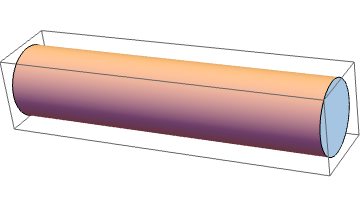
Let us consider a heat conduction problem for a straight bar of uniform cross section and homogeneous material. With appropriate Cartesian coordinate system, the bar of length ℓ is oriented in the horizontal x-direction from x = 0 to x = ℓ. Suppose further that the sides of the bar are perfectly insulated so that no heat passes through them. We also assume that the cross-sectional dimensions are so small that the temperature u can be considered constant on any given cross section. Then u is a function of the axial coordinate x and the time t.
Graphics3D[Cylinder[{{0,0,0},{3,0,0}}, 1/3]]
The variation of temperature in the bar is governed by the partial differential equation, called the heat equation or diffusion equation:
In general, a positive coefficient α>0, known as the thermal diffusivity, may depend on spatial variables, temperature, and pressure. However, we assume the thermal diffusivity to be constant in our problems, for simplicity. The parameter α depends only on the material from which the rod is made and is defined by
In order to determine a unique solution to the heat transfer equation, we need to specify its initial temperature at t=0 and boundary conditions at end points.
It is assumed that the initial temperature distribution in the bar is known
where f is some given function. The physics of the problem dictates that this function must also satisfy some regularity conditions to match the temperature at the boundary. However, sometimes the corresponding initial boundary value problem (IBVP for short) can be considered without these regularity conditions with the expense of not uniform convergence of solution.
The general solution of a partial differential equation is very sensitive to the boundary conditions. As such, the same equation may posses different properties under different sets of boundary conditions. In this section, we illustrate this fact by examining one dimensional heat conduction problems with different sets of boundary conditions. First, we consider a long metal bar of length ℓ which is much longer than it is thick. This means that we can treat the distribution of heat as a function of just one spatial variable x ∈ [0, ℓ] and time variable t. The bar is assumed to be insulated along its length so that it can only gain and lose heat through its ends. This means that the temperature distribution u(x, t) depends only on these two variables.
Keep in mind that, throughout this section, we will be solving the same one-dimensional homogeneous partial differential equation, Eq.\eqref{EqBheat.1}, which is called the diffusion equation (also known as the heat transfer equation).
The heat conduction equation can now be paired up with a set of boundary conditions, of which we consider three most common types:
The second type of boundary conditions or Neumann conditions ( named after Carl Neumann) when the heat flow (in general, the surface heat flux) is specified
The third type of boundary conditions or mixed boundary conditions usually include the following two cases.
On one part of the boundary the temperature is specified (the Dirichlet conditions), while on another part the normal derivative is specified (Neumann conditions).
When we observe convective heat transfer at the boundary
where κ is the thermal conductivity of the material (with units W/(m K)), h is the convection heat transfer coefficient (with unites Watt/m² -K), and A is the surface area (units m²). The convection heat transfer coefficient is sometimes referred to as a film coefficient. It represents the thermal resistance of a relatively stagnant layer of fluid or air between a heat transfer surface and the fluid medium. It can also be defined through the Nusselt number:
\( \displaystyle h = \left( Nu \cdot \kappa \right) /L , \) where Nu is the Nusselt number, κ is the thermal conductivity, and L is the characteristic length.
Diffusion equation with the Dirichlet boundary condition
Consider a heat transfer problem for a thin straight bar (or wire) of uniform cross section and homogeneous material. Let the x-axis be chosen along the axis of the bar, and let x=0 and x=ℓ denote the ends of the bar. Suppose further that the lateral surface of the rod are perfectly insulated so that no heat transfers through them. We also assume that the cross-sectional dimensions are so small that the temperature u can be considered constant on any cross section. Then u is a function only of the axial coordinate x and the time t.
Assuming that no heat is being generated within the rod, the variation of temperature in it is governed by the partial differential equation (of parabolic type):
where α > 0 is a constant known as the thermal diffusivity.
In addition, we assume that the ends x=0 and x=ℓ of the rod are held at fixed temperatures. More over, these temperatures are assumed to be zeroes, u(0,t) = 0℃ and u(ℓ,t) = 0℃ during all heat conduction process (for all t). This requirement is essential for the method of separation of variables that will be used to obtain the solution of Eq.\eqref{EqBheat.1}. In the following section, it will be shown how to bypass the homogeneity of the boundary conditions.
For now, we consider the following boundary conditions:
As previously stated, the regularity conditions are dictated by the physics of the problem.
They consist of two parts: the first part requires the matching for the initial temperature with the homogeneous boundary conditions to maintain the continuity of the temperature distribution inside the rod. This condition can be disregarded because it does not affect the solvability of the IBVP. However, violation of this condition makes the given problem ill-posed and its numerical approximation may suffer instability or the Gibbs phenomena. The second condition is almost always satisfied because temperature approaches zero with time due to dissipation of energy.
The following animation gives the temperature distribution in a finite bar subject to homogeneous Dirichlet boundary conditions:
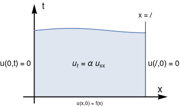
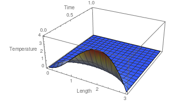
The fundamental problem of heat conduction is to find u(x, t) that satisfies the heat equation and subject to the boundary and initial conditions.
Under some light conditions on the initial function f, the formulated initial boundary value problem has a unique solution. This problem can be considered as a boundary value problem in xt-plane (see figure below). The solution u(x, t) of the heat equation is sought in the semi-infinite strip 0 < x < ℓ, t > 0, subject to the requirement that u(x, t) must assume a prescribed values at each point on the boundary of this strip.
Boundary value problem for the heat conduction equation.
As it is seen from the figure, the boundary for the xt-domain is not smooth because it has two corner points (0,0) and (ℓ,0). In this case, we have to impose the regularity conditions to make the corresponding IBVP well-posed.
Note that the equation and boundary conditions are homogeneous---only under these assumptions the separation of variables method is applicable. This gives us a way to seek its solution as superposition of some nontrivial solutions of the auxiliary problem:
So we seek nontrivial (which means not identically zero) solutions of the above auxiliary problem that are represented as a product of two functions:
\[
u(x,t) = X(x)\, T(t) ,
\]
where functions X = X(x) depends only on spatial variable x and T = T(t) depends on time variable t. Substituting this product into the heat equation, we get
in which the variables are separated. Since the left hand side depends only on time variable t, the right side depends on spatial variable x, and these variables are independent, these functions could be equal only when they are constant. Denoting this constant of separation as −λ, we arrive at two ordinary differential equations:
Considering together the differential equation for X(x) and the homogeneous boundary conditions, we obtain the familiar Sturm--Liouville problem that we discussed previously:
Hence, T(t) = Tn(t) is proportional to the exponent \( \exp \left\{ - \frac{\alpha\, n^2 \pi^2 t}{\ell^2} \right\} , \ n=1,2,\ldots . \) Multiplying functions Tn and Xn, we obtain for each n partial nontrivial solution of the heat equation satisfying the homogeneous boundary conditions of Dirichlet type:
Each partial nontrivial solution un(x, t) satisfies the heat conduction equation \eqref{EqBheat.1} and the homogeneous boundary conditions. Obviously, an arbitrary linear combination of these functions will also satisfy the homogeneous heat equation and boundary conditions (in our case, they are of Dirichlet type).
Now we apply the principle of superposition by seeking a solution to the given IBVP that is a linear combination of all partial nontrivial solutions
Assuming that the series \eqref{EqBheat.3} converges uniformely (this condition is required to interchange the order of limit and summation), the the sum function u(x, t) satisfies the partial differential equation \( u_t = \alpha\, u_{xx} \) and homogeneous boundary conditions u(0,t) = 0 and u(ℓ,t) = 0 because the individual terms un have the same property. It remains only to satisfy the initial condition
So if we can move the limit under the sign of summation (this is possible when the series converges uniformly), then what is remained to do is to determine
the coefficients cn so that the identity
holds
In other words, we have to determine coefficients cn so that the Fourier sine series converges to the initial temperature distribution f(x) for 0<x<ℓ. According to Euler--Fourier formula, we have
All that remains is to investigate whether the Fourier sine series representation \eqref{EqBheat.3} of u(x, t) can satisfy the heat equation, ∂u/∂t = α ∂²u/∂x². To do that, we must differentiate
the Fourier sine series that leads to justification of performing term-by-term differentiation. What is important for it is to remember that the heat equation must be verified in the open domain 0 < x <∞, 0 < t <∞.
The expression \eqref{EqBheat.3} for the temperature is not easy to analyze, but the negative exponential factor in each term of the series causes the series to converge if the coefficients \eqref{EqBheat.5} do not grow exponentially. If the initial temperature is represented by a function f(x) of bounded variation, then these coefficients decrease and the total series \eqref{EqBheat.3} converges quite rapidly for t ≥ t0 > 0.
This tells us that we can differentiate term by term of u(x, t) any times in the open domain 0 < x <∞, 0 < t <∞. In particular, the series
The solution series \eqref{EqBheat.3} converges actually in the semi-open domain 0 ≤ x <∞, 0 < t <∞. So the boundary conditions are also satisfies because the following relations hold
For small t, the series solution \eqref{EqBheat.3} may converge, but not uniformly, and proving the validity of the initial condition can be challengeable.
provides a good approximation to the true solution in the domain t ≥ t0 > 0 because every term un(x, t) satisfies exactly the heat conduction equation and the boundary conditions, and the the exponential tail of the remainder can be ignored. Therefore, the truncated series can be used for actual approximation to the solution for the moderate values of t, but it loses its fast convergence for small t, which requires additional attention.
If the initial temperature function f(x) is twice differentiable on the interval [0, ℓ] and f(0) = f(ℓ) = 0, then we can integrate by parts to obtain
This relation shows that the coefficients cn decay as n−2. So the series
\( \sum_n c_n X_n (x) \) converges uniformly for x ∈ [0, ℓ]. Therefore, we can interchange the limit as t → 0 and summation.
Example 1A:
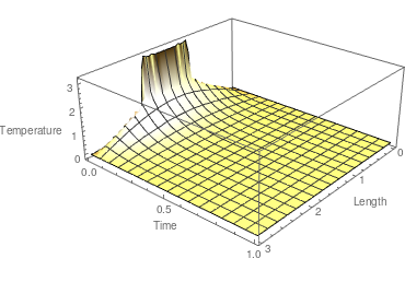
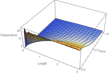
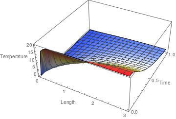
Consider a uniform rod of length ℓ = 3 meters long, insulated on sides, with thermal diffusivity 9.
If initially the rod has a constant temperature of 20℃, but homogeneous Dirichlet boundary conditions are maintained, we come to the following IBVP:
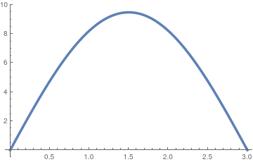
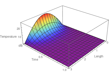
The temperature in the rod satisfies the heat conduction equation \eqref{EqBheat.1} with ℓ = 3 and initial temperature f(x) = 20 for 0 < x < 3. Thus, from Eq.\eqref{EqBheat.3}, the solution is
The series solution converges rapidly in the domain t ≥ t0 > 0, but the initial conditions are difficult to verify because the series does not converge uniformly for small t and we cannot set t = 0 under the sign of summation because it converges conditionally.
Now we demonstrate how this problem can be solved with Mathematica. Firs, we define the heat partial differential equation that represents the
temperature in the bar:
heatEq = D[u[x, t], t] == 9 * D[u[x, t], {x, 2}]
\( u^{(0,1)}[x, t] = 9\,u^{(2,0)}[x, t] \)
Then we solve the heat equation with the appropriate boundary conditions
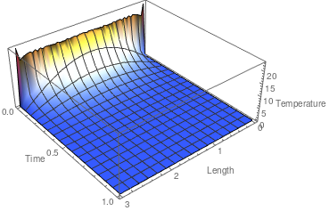
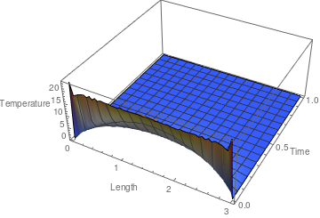
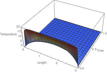
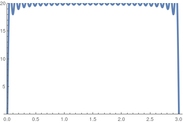
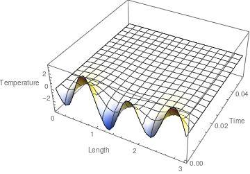
As it is seen from the graph, there are ripples near the edge t = 0, which indicates poor convergence of the series. This is a confirmation that the given initial boundary value problem is ill-posed; so the corresponding numerical calculations must be done with care. The Gibbs phenomenon becomes clear when plotting the graph from a different perspective.
The graph reveals a Gibbs phenomena near the edge t = 0. We take the truncated sum with 31 terms and plot it.
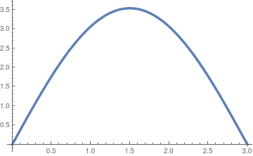
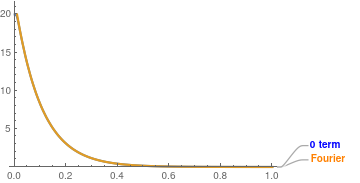
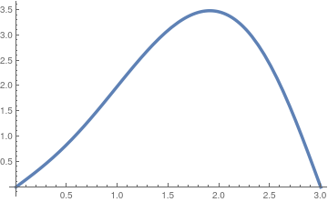
We plot temperature as a function of the position across the bar at
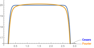
different time values. First, we compare truncated versions of regular Fourier approximation and its Cesàro counterpart for tiny t = 0.001.
We put two temperature profiles at t = 0.001 together for comparison,
Of course, Mathematia complains that the exponential terms are too small for actual calculations. Therefore, 30-term approximation is not needed and first few terms is sufficient for accurate approximations.
Temperature distribution at t = 0.1.
Temperature distribution at t = 0.2.
Temperature distribution at t = 2.1.
In order plot the temperature as a function of the time at different position
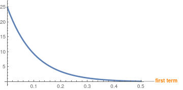
values along the bar, we compare its distribution with just first term
Example 1B:
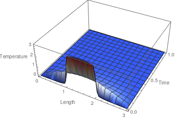
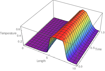
Consider conduction of heat in a rod 3 meters in length whose ends are maintained at 0℃. Initially, the rod was heated to 20℃ inside the interval 1 < x < 2. This yields the initial boundary value problem:
The initial temperature distribution u(x, 0+) satisfies the regularity conditions on the boundary x = 0 and x = ℓ. However, it is a piecewise continuous function and its sine Fourier expansion converges not uniformely exhibiting the Gibbs phenomenon.
For small t, the series converges conditionally, which resembles the alternating series \( \sum_k \frac{(-1)^k}{2k+1} = \frac{\pi}{4} . \) Alternating series are not easy to numerically evaluate. For example, the hundred terms give only two correct decimal places:
N[Sum[(-1)^k /(2*k + 1) , {k, 0, 100}]]
0.787873
But the true value is
N[Pi/4]
0.785398
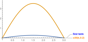
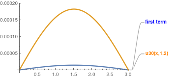
For plotting, we extract the truncation sum with 30-terms as an approximation to the true solution and then compare it with the first term
Both figures, s0(x, t) at the left and u30(x, t) at the right, exhibit similar behavior for moderate t.
The ripples near the edge t = 0 in the right-hand side figure indicate the Gibbs phenominon because of poor convergence of the series. To get rid of them, we apply >Cesàro summation.
We take the ;Cesàro truncated sum with 31 terms and plot it. As it is clearly seen, there is no Gibbs phenomenon.
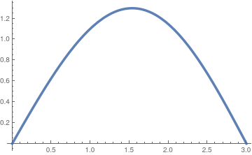
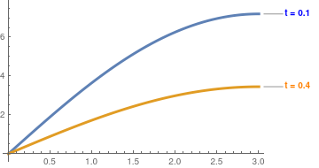
We plot temperature as a function of the position across the bar at different time values. In order to understand the influence of the first (main) term, we plot truncated versions of regular Fourier approximation and the corresponding first term for several values of t.
Starting with t = 0.01, there is no visible difference in regular Fourier summation and corresponding Cesàro approximation.
Of course, Mathematia complains that the exponential terms are too small for actual calculations. Therefore, 30-term approximation is not needed and first few terms is sufficient for accurate approximations starting at t = 1.
Temperature distribution at t = 0.2.
Temperature distribution at t = 1.2.
Temperature distribution at t = 2.2.
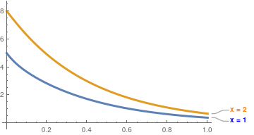
In order plot the temperature as a function of the time at different position
values along the bar, we compare its distribution with just first term.
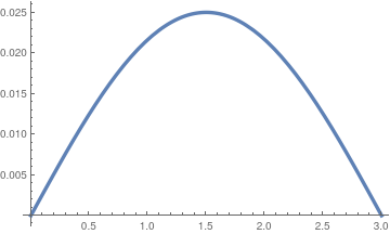
-((54 (2 n \[Pi] +
4 n \[Pi] Cos[n \[Pi]] + (-6 + n^2 \[Pi]^2) Sin[n \[Pi]]))/(
n^4 \[Pi]^4))
Since the initial temperature distribution u(x, 0+)
is a continuous function and
satisfies the regularity conditions at the boundary. Therefore, the corresponding series solution converges uniformely for t ≥ 0.
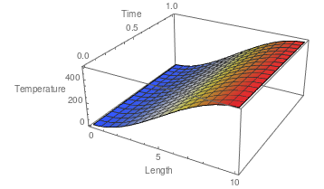
In the given problem, we consider a bar of length ℓ = 3 with thermal diffusivity α = 9. We can find its solution using the general formula \eqref{EqBheat.3} and evaluate coefficients according to \eqref{EqBheat.5}. However, we don't need to go over this tedious procedure because
the initial condition function u(x, 0+) = f(x) is a linear combination of the eigenfunctions. Since the sine Fourier series expansion is unique for any square integrable function f ∈ 𝔏², this function f(x) is its Fourier series for itself:
This allows us to identify the coefficients to be all zeroes except two indices: c3 = 1 and c6 = −3.
Using the superposition principle, the solution of the given IBVP can be obtained by adding together two simpler solutions corresponding n = 3 and n = 6
obtained by the product method:
Let us consider the situation where two ends of the bar are also sealed with perfect insulation so that no heat can escape to the outside environment (recall that the side of the bar is always perfectly insulated in the one-dimensional assumption), or vice versa. The new boundary conditions follow from the Fourier’s law of heat transfer that the rate of heat transfer is proportional to negative temperature gradient:
\[
\frac{\mbox{Rate}\ \mbox{ of }\ \mbox{ heat}\ \mbox{ transfer}}{\mbox{area}} = -\kappa\,\nabla u = - \kappa\,\frac{\partial u}{\partial x} ,
\]
where κ is the thermal conductivity. In other words, heat is transferred from areas of high temperature to low temperature.
\[
\left. \frac{\partial u}{\partial x} \right\vert_{x=0} = 0 \qquad \mbox{and} \qquad \left. \frac{\partial u}{\partial x} \right\vert_{x=\ell} = 0,
\]
reflecting the fact that there will be no heat transferring, spatially, across the points x = 0 and x = ℓ. The heat conduction problem becomes the initial-boundary value problem below.
The first step is to temporarily disregard the initial condition (because it is non-homogeneous) and consider an auxiliary boundary value problems. Next, we apply the separation of variables for the function u(x, t) = X(x) T(t )that leads to two ordinary differential equations
To satisfy the Neuman boundary conditions, we have to set c2 = 0. Then function \( X(x) = c_1 \) is a solution of the differential equation \( X'' (x) + 0\cdots X(x) = 0 \) and automatically satisfies both Neuman boundary conditions. Therefore, any constant solution X(x) = c1 ≠ 0 is an eigenfunction.
Assuming λ to be positive, the general solution of the differential equation for X(x) becomes
with some constants c1 and c2. Taking derivative \( X'(x ) = \sqrt{\lambda} \left[ -c_1 \sin \left( \sqrt{\lambda}\,x \right) + c_2 \cos \left( \sqrt{\lambda}\,x \right) \right] , \)
and substituting into the boundary conditions, we get
Since λ is positive (by assumption), the only choice we have is to set
\( \sin \left( \sqrt{\lambda}\,\ell \right) =0 \) because we cannot affort a trivial solution by setting c2 = 0. Then we obtain the eigenvalues and corresponding eigenfunctions:
We included n = 0 because λ = 0 is an eigenvalue with a constant as an eigenfunction. Every auxiliary function un(x, t) = Xn(x) is a solution of the homogeneous heat equation \eqref{EqBheat.1} and satisfy the homogeneous Neumann boundary conditions. Thereofre, any their linear combination will also a solution of the heat equation subject to the Neumann boundary conditions.
Hence we expect the sum over all auxiliary partial nontrivial solutions will be a solution of our given IBVP provided that the infinite series converges. So we seek the solution in the form:
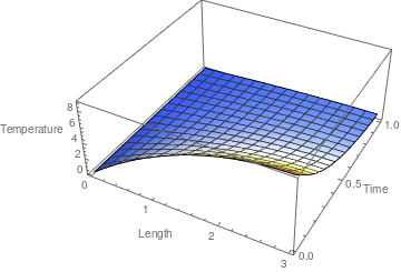
The initial temperature f(x) = x²(15 −x) satisfies the regularity conditions: \( f' (0) = f' (10) = 0 . \) Therefore, we expect that the given IBVP to be well-posed.
Since its solution is available from Eq.\eqref{EqBheat.6}, we get the explicit fornmula for it:
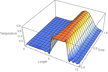
where H(x) is the Heaviside function. Although the initial temperature function satisfies the regularity conditions, it is piecewise continous. Therefore, we expect to observe a Gibbs phenomenon dues to poor convergence of the corresponding solution series.
The series converges uniformly in any domain t ≥ t0 > 0 because of the expobnentially decayed multiple containing t. However, when t is close to zero, the series converges conditionally and the initial condition is not easy to satisfy. To suppress the Gibbs phenomenon, we apply the Cesàro summation. First, we define a 31-term approximation
In the given problem, we consider a bar of length ℓ = 10 with thermal diffusivity α = ¼. We can find its solution using the general formula \eqref{EqBheat.6} and evaluate coefficients according to \eqref{EqBheat.7}. However, we don't need to go over this tedious procedure because
the initial condition function u(x, 0+) = f(x) is a linear combination of the eigenfunctions. Since the cosine Fourier series expansion is unique for any square integrable function f ∈ 𝔏², this function f(x) = cos(πx) −2 cos(2πx)is its Fourier series for itself:
This allows us to identify the coefficients to be all zeroes except two indices: c10 = 1 and c20 = −3.
Using the superposition principle, the solution of the given IBVP can be obtained by adding together two simpler solutions corresponding n = 3 and n = 6
obtained by the product method:
Simple Mixed boundary condition for the diffusion equation
We consider two initial boundary value problems with Dirichlet's condition (when temperature is prescribed to be zero) on one end and Neumann condition (which is equivalent insulation) on another end.
When regularity conditions are satisfied, the given initial boundary value problem (IBVP for short) is well-posed. However, when the conditions at end points do not meet or the initial temperature is modelled by a ppiecewise continuous function, the IBVP can also be solved, but it becomes ill-posed and numerical calculations must be done with care.
Disregarding the initial condition, we obtain an auxiliary boundary value problem. We seek for its non-trivial solutions that are represented as the product u(x, t) = X(x) T(t) of two functions, X(x) and T(t), each of which depends on single independent variable. Substituting this form into the heat equation, we get
Its left-hand side depends on time variable t, but the right-hand side depends on spatial variable x that are independent. Therefore, this equation holds only when both sides are constants. As usual, we denot this constant as −λ. This give two differential equations containing a parameter λ (which is unknown yet):
It can be shown that the Sturm--Liouville problem has nontrivial solutions only for positive values of parameter λ. Assuming this, we obtain the general solution to the differential equation
\( X'' (x) + \lambda\,X(x) =0 \) to become
To satisfy the boundary condition at x = 0 we have to set c₁ = 0 and obtain \( X(x) = c_2 \sin \left( \sqrt{\lambda}\,x \right) . \) An arbitrary constant c₂ ≠ 0 in order to avoid the identically zero solution, so it can be dropped. Next substitution of this function into the boundary condition at x = ℓ, we get
with some arbitrary constant cn. Multiplying Tn(t) and Xn(x), we find partial nontrivial solutions to our auxiliary boundary value problem. Upon summing all these partial nontrivial solutions, we represent the required solution as an infinite series
Every term in this infinite series satisfies the heat conduction equation and both boundary conditions.
Assuming that this series converges, we extend this statement for the series. Now substituting u(x, t) into the initial condition,
This identity is valid only when the limit can be evaluated under the sum sign (which is true when the series converges uniformly). It is not our case, and we apply the Cesàro summation to prove the validity of interchanging the order of limiting procedure and summation.
Note the the regularity conditions are valid, so the given problem is well-posed. We seek its solution as the sum of all partial nontrivial solutions (assuming that the series converges uniformely):
In order to satisfy the initial conditions, we take the limit as t approaches zero; assuming that the series converges uniformly. Then we apply the limit to every term under the summation sign and obtain
Problem ND:
We consider a heat transfer problem for a rod of length ℓ
with Dirichlet's condition (when temperature is prescribed to be zero) on right end x = ℓ and Neumann's condition (which is equivalent insulation) on another end x = 0.
So the left end x = 0 is maintained with a constant (zero) temperature, while on the another end x = ℓ there is a convection heat transfer with surrounded air of temperature T ∞. Since we are in the section to illustrate separation of variables method, we make a simplified assumption that T ∞ is zero. This leads to the following (simplified boundary conditions:
where γ is a positive constant. In order to apply the separation of variables method, we temporarily disregard the initial condition (because it it is nonhomogeneous) and obtain the auxiliary boundary value problem
Assuming that this problem has a solution represented as a product of two functions, u(x, t) = X(x) T(t), we obtain upon its substitution into the heat equation that
Assuming that λ is posityive (for other values of λ, the corresponding Sturm--Liouville problem has no nontrivial solution), we obatian solution that satisfies the boundary condition at x = 0:
Let μn (n = 1, 2, …) be a sequence of positive zeroes of Eq.\eqref{Eqconvert.2} (μ = 0 is not an eigenvalue because the corresponding eigenfunction is identically zero). Then eigenvalues and eigenfunctions of the Sturm--Liouville problem are
where \( \displaystyle \lambda_n = \left( \frac{\mu_n}{\ell} \right)^2 , \) and μn are positive roots of the transcedent equation tan (μ) + (γ/ℓ) μ = 0, form a complete orthogonal set on [0, ℓ].
This states that the right end of the bar radiates heat to its surroundings at a rate proportional to its current temperature. The left end x = 0 is maintained at zero temperature.
■
Maple (with animation):
https://www.maplesoft.com/applications/view.aspx?SID=3601&view=html
Example:
■
Example:
We are going to find the temperature u(x,t) at any time t is a metal rod 9 cm long, insulated on the sides. It is assumed that the end points are maintained at 0°C throughout. Initial temperature at t = 0 is specified along a semi-linear law described explicitly later.
The temperature in the rod satisfies the heat conduction problem and we have to consider the initial
boundary value problem
where α² = 111 and ℓ = 30. Since the ratio ℓ²/α² has units of time, it is convenient to use this quantity to define a dimensionless time variable τ = (α²/ℓ²)t, with α² = 111. Then the given heat conduction problem will be written in dimensionless variables as
Example:
Let a metallic rod of 50 cm long be heated to the temperature
\[
f(x) = \begin{cases} 0 , & \ \mbox{ if } 0 \le x < 20 ,
40, & \ \mbox{ if } 20 < x < 40, \\
0 , & \ \mbox{ if } 40 < x < 50. \end{cases}
\]
Suppose that the rod is insulated on all sides, including end points. Then the temperature u(x,t) inside the rod is the solution of the following initial boundary value problem (IBVP):
Return to Mathematica page
Return to the main page (APMA0340)
Return to the Part 1 Matrix Algebra
Return to the Part 2 Linear Systems of Ordinary Differential Equations
Return to the Part 3 Non-linear Systems of Ordinary Differential Equations
Return to the Part 4 Numerical Methods
Return to the Part 5 Fourier Series
Return to the Part 6 Partial Differential Equations
Return to the Part 7 Special Functions