Preface


In this section, we discuss the initial boundary value problems (IBVPs for short) for wave equation. Although these problems can be solved using the reflection principle or the unified transform method, the main tool in our presentation is the separation of variables, also known as the Fourier method.

Return to computing page for the first course APMA0330
Return to computing page for the second course APMA0340
Return to Mathematica tutorial for the first course APMA0330
Return to Mathematica tutorial for the second course APMA0340
Return to the main page for the first course APMA0330
Return to the main page for the second course APMA0340
Return to Part VI of the course APMA0340
Introduction to Linear Algebra with Mathematica

Strings that are used in musical instruments (guitar, piano, violin, arpha, and so on) are typical examples of incompressible elastic strings. Since displacements of these strings are small compared to the total length, we can assume that musical strings vibrate within a plane, for which we use the Cartesian coordinate system. Let us consider a taut string of length ℓ that is stretched between two fixed points. Let the abscissa is chosen to lie along the string and let x = 0 and x = ℓ denote the ends of the string that are assumed to be fixed. Let u(x, t) denote the vertical displacement experienced by the string at the point x at time t. If damping effects, such as air resistance, are neglected, and if the amplitude of the motion is small compared to the string length, then u(x, t) satisfies the partial differential equation, known as the wave equation
\[ \frac{\partial^2 u}{\partial t^2} = c^2 \frac{\partial^2 u}{\partial x^2} \qquad \mbox{or for short} \qquad u_{tt} = c^2 u_{xx} . \]

Initial Boundary Value Problems for Wave Equation


We are now in a position to solve the general initial boundary value problem for the wave equation subject to homogeneous boundary conditions of the first type (Dirichlet's conditions are chosen for simplicity):

\begin{equation} \label{EqIBVP.1} \left\{ \begin{array}{ll} \ddot{u} = c^2 u_{xx} , & 0 < x < \ell , \quad 0<t<t^{\ast} <\infty ; \\ u(0,t) = u(\ell ,t) =0, & 0 < t< t^{\ast} < \infty ; \\ u(x,0) = d(x) , \quad \dot{u} (x,0) = v(x) ,\quad & 0<x<\ell . \end{array} \right. \end{equation}
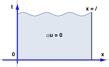
The given initial boundary value problem \eqref{EqIBVP.1} models transverse vibrations of an elastic string of length ℓ with two endpoints fixed. Here d(x) and v(x) are initial vertical displacement and velocity of the string, respectively. Alternatively, it can be considered as a boundary value problem in the semi-infinite strip 0 < x < ℓ,    t > 0 of the xt-plane. One condition (boundary) is imposed at each point on the semi-infinite sides, and two (initial conditions) are imposed at each point on the finite horizontal base.

     
fil = Plot[{1.3 + 0.05*Sin[20*x], 0}, {x, 0, 1.0}, Filling -> {1 -> {2}}, Ticks -> None, PlotRange -> All];
har = Graphics[{Arrowheads[0.06], Thickness[0.01], Blue, Arrow[{{-0.2, 0}, {1.2, 0}}]}];
var = Graphics[{Arrowheads[0.06], Thickness[0.01], Blue, Arrow[{{0, -0.1}, {0, 1.6}}]}];
line = Graphics[{Thick, Black, Line[{{1.0, 0}, {1.0, 1.35}}]}];
t1 = Graphics[{Black, Text[Style["t", Bold, 18], {-0.07, 1.5}]}];
t2 = Graphics[{Black, Text[Style["x = \[ScriptL]", Bold, 18], {1.0, 1.45}]}];
t3 = Graphics[{Black, Text[Style["x", Bold, 18], {1.15, 0.15}]}];
t4 = Graphics[{Black, Text[Style["\[Square]u = 0", Bold, 18], {0.5, 0.7}]}];
t5 = Graphics[{Black, Text[Style["0", Bold, 18], {-0.05, 0.15}]}];
Show[fil, har, var, line, t1, t2, t3, t4, t5]
       Domain            Mathematica code

We are going to solve the given problem \eqref{EqIBVP.1} using separation of variables method. As usual in this case, we consider an auxiliary problem that consists of the wave equation and homogeneous boundary conditions:

\[ \left\{ \begin{array}{ll} \ddot{u} = c^2 u_{xx} , & 0 < x < \ell , \quad 0<t<t^{\ast} <\infty ; \\ u(0,t) = u(\ell ,t) =0, & 0 < t< t^{\ast} < \infty ; \\ \end{array} \right. \]
We seek its partial nontrivial solutions in the form \( u(x,t) = X(x)\,T(t) . \) Substituting this function into the wave equation gives
\[ \frac{X'' (x)}{X(x)} = \frac{\ddot{T}(t)}{c^2 T(t)} = -\lambda . \]
Separation of variables yields
\[ \begin{split} \ddot{T}(t) + c^2 \lambda\, T(t) &=0 , \\ X'' (x) + \lambda \,X(x) &=0 . \end{split} \]
Similarly to the previous sections (see Example 2 in section 2.5i and section on boundary value problems for the heat equation), we substitute \( u(x,t) = X(x)\,T(t) \) into the boundary conditions to obtain X(0) = 0 and X(ℓ) = 0. The differential equation together with these boundary conditions constitute the Sturm--Liouville problem:
\begin{equation} \label{EqIBVP.2} X'' (x) + \lambda \,X(x) =0, \qquad X(0) =0, \quad X(\ell ) =0 . \end{equation}
Of the usual three possibilities for the parameter, λ = 0, λ = -α² < 0, and λ = α² > 0, only the last choice leads to nontrivial solutions. Corresponding to λ = α² > 0, with α > 0, the general solution to the differential equation \( X'' (x) + \alpha^2 \,X(x) =0 \) is
\[ X(x) = c_1 \cos \alpha x + c_2 \sin \alpha x . \]
The boundary conditions X(0) = 0 and X(ℓ) = 0 dictate that c1 = 0 and \( c_2 \sin \alpha \ell =0 . \) The latter equation implies that \( \sin \alpha \ell =0 \) because otherwise c2 = 0 forces to obtain a trivial solution. Since we cannot affort vanishing c2, we have to choose α to be
\[ \alpha = \sqrt{\lambda} = \frac{n\pi}{\ell} , \qquad n=1,2,3,\ldots . \]
Therefore, we obtain the eigenvalues and corresponding eigenfunctions:
\begin{equation} \label{EqIBVP.3} \lambda_n = \left( \frac{n\pi}{\ell} \right)^2 , \qquad X_n (x) = \sin \frac{n\pi x}{\ell}, \qquad n=1,2,3,\ldots . \end{equation}
The general solution of the second order differential equation \( \ddot{T} + c^2 \lambda_n T(t) =0 \) becomes
\[ T_n (t) = A_n \cos \frac{cn\pi t}{\ell} + B_n \sin \frac{cn\pi t}{\ell} , \qquad n=1,2,3,\ldots . \]
Since the eigenfunction \( X_n (x) = \sin \frac{n\pi x}{\ell} \) can be multiplied by any nonzero constant, we find partial nontrivial solutions of our auxiliary problem:
\begin{equation} \label{EqIBVP.4} u_n (x,t) = X_n (x) \, T_n (t) = \sin \frac{n\pi x}{\ell} \left( A_n \cos \frac{cn\pi t}{\ell} + B_n \sin \frac{cn\pi t}{\ell} \right) , \qquad n=1,2,3,\ldots . \end{equation}
Finally, we represent the required solution of the given initial boundary value problem as the sum of all partial nontrivial solutions
\begin{equation} \label{EqIBVP.5} u(x,t) = \sum_{n\ge 1} u_n (x,t) = \sum_{n\ge 1} X_n (x) \, T_n (t) = \sum_{n\ge 1} \sin \frac{n\pi x}{\ell} \left( A_n \cos \frac{cn\pi t}{\ell} + B_n \sin \frac{cn\pi t}{\ell} \right) . \end{equation}
To satisfy the initial conditions, we assume that we can apply the limit as t → 0 under the sign of summation and then use the trigonometric formulas sin(0) = 0 and cos(0) = 1. Setting t = 0, we get from the initial condition u(x, 0) = d(x) that
\[ u(x,0) = d(x) = \sum_{n\ge 1} u_n (x,0) = \sum_{n\ge 1} A_n X_n (x) = \sum_{n\ge 1} A_n \sin \frac{n\pi x}{\ell} . \]
Since the latter series is just Fourier sine series (see formula (2) in section on even and odd functions) for d(x), we can write
\[ A_n = \frac{2}{\ell} \int_0^{\ell} d(x)\, \sin \frac{n\pi x}{\ell} \,{\text d} x , \qquad n=1,2,3,\ldots . \]
To determine Bn, we differentiate the general solution with respect to t and the set t = 0:
\[ \begin{split} \frac{\partial u}{\partial t} &= \sum_{n\ge 1} \left( -A_n \frac{cn\pi}{\ell} \, \sin \frac{cn\pi t}{\ell} + B_n \frac{cn\pi}{\ell}\, \cos \frac{cn\pi t}{\ell} \right) \sin \frac{n\pi x}{\ell} , \\ \left. \frac{\partial u}{\partial t} \right\vert_{t=0} &= v(x) = \sum_{n\ge 1} B_n \frac{cn\pi}{\ell}\, \sin \frac{n\pi x}{\ell} . \end{split} \]
For this last sine Fourier series to be expansion of v(x), the total coefficient of sine must be given by
\[ B_n \frac{cn\pi}{\ell} = \frac{2}{\ell} \int_0^{\ell} v(x)\, \sin \frac{n\pi x}{\ell} \,{\text d} x , \]
from which we obtain
\[ B_n = \frac{2}{n\pi c} \int_0^{\ell} v(x)\, \sin \frac{n\pi x}{\ell} ,{\text d} x , \qquad n=1,2,3,\ldots . \]
Recall that the constant c appearing in the solution of the initial boundary value problem is given by \( c= \sqrt{T/\rho} , \) where ρ is mass per unit length and T is the magnitude of the tension in the spring. When T is large enough, the vibrating string produces a musical sound. This sound, according to the solution
\begin{equation} \label{EqIBVP.6} u(x,t) = \sum_{n\ge 1} u_n (x,t) , \end{equation}
is the result of sum (superposition) of standing waves or normal modes.
Submit
Each normal mode can be written as
\begin{equation} \label{EqIBVP.7} u_n (x,t) = C_n \sin \left( \frac{n\pi c}{\ell} \,t + \phi_n \right) \sin \frac{n\pi x}{\ell} , \end{equation}
where
\[ C_n = \sqrt{A_n^2 + B_n^2} , \qquad \sin \phi_n = A_n /C_n \quad\mbox{or}\quad \cos \phi_n = B_n / C_n . \]
For \( n= 1,2,3,\ldots \) the standing waves are essentially the graphs of sine function \( \sin \frac{n\pi x}{\ell} \) with a time-varying amplitude given by
\[ C_n \sin \left( \frac{n\pi c}{\ell} \,t + \phi_n \right) . \]
Alternatively, we see from the formula for the normal mode un(x,t) that at a fixed value of x this function represents simple harmonic motion with amplitude \( C_n \sin \frac{n\pi x}{\ell} \) and frequency fn = nc/(2ℓ). In other words, each point on a standing wave vibrates with a different amplitude but with the same frequency. The spacial period 2ℓ/n is called the wavelength of the mode of frequency nπc/ℓ. As x runs from 0 to ℓ, the argument of \( \sin \frac{n\pi x}{\ell} \) runs from 0 to nπ, which is n half-periods of sine function. The mode corresponding n = 1,
\[ u_1 (x,t) = C_1 \sin \left( \frac{c\pi}{\ell}\,t + \phi_1 \right) \sin \frac{\pi x}{\ell} , \]
is called the first standing wave, the first normal mode, or the fundamental mode of vibration, and its frequency is called the fundamental frequency:
\[ f_1 = \frac{c}{2\ell} = \frac{1}{2\ell} \sqrt{\frac{T}{\rho}} . \]
The fundamental frequency or first harmonic is directly related to the pitch (or note) produced by a string instrument. It is apparent that the greater the tension on the string, the higher the pitch of the sound. The frequencies fn of the other normal modes, which are integer multiples of the fundamental frequency, are called overtones.

Standing wave patterns are wave patterns produced in a medium when two waves of identical frequencies interfere in such a manner to produce points along the medium that always appear to be standing still. These points that have the appearance of standing still are referred to as nodes. There are several frequencies with which a string can be vibrated to produce the patterns. Each frequency is associated with a different standing wave pattern. These frequencies and their associated wave patterns are referred to as harmonics. The two individual waves are drawn in blue and green and the resulting shape of the medium is drawn in black.

Example 1:

Solve the initial boundary value problem:

\[ \left\{ \begin{array}{ll} \ddot{u} = 9 \,u_{xx} , & 0 < x < 50, \quad 0<t<t^{\ast} <\infty ; \\ u(0,t) = u(50,t) =0, & 0 < t< t^{\ast} < \infty ; \\ u(x,0) = 3\,\sin (2\pi x) , \quad \dot{u} (x,0) = 5\,\sin (3\pi x) ,\quad & 0<x<50. \end{array} \right. \]
The given initial boundary value problem is a particular case of IBVP \eqref{EqIBVP.1} with ℓ = 50, c = 3, and the initial functions \( d(x) = 3\,\sin (2\pi x) , \quad v (x) = 5\,\sin (3\pi x) . \) It was solved previously and its solution formula \eqref{EqIBVP.7} is known
\[ u(x,t) = \sum_{n\ge 1} \sin \frac{n\pi x}{50} \left( A_n \cos \frac{3n\pi t}{50} + B_n \sin \frac{3n\pi t}{50} \right) , \]
where
\[ \begin{split} A_n &= \frac{1}{25} \int_0^{50} 3\,\sin (2\pi x) \,\sin \frac{n\pi x}{50} \,{\text d}x , \qquad n=1,2,\ldots , \\ B_n &= \frac{2}{3n\pi} \int_0^{50} 5\,\sin (3\pi x) \,\sin \frac{n\pi x}{50} \,{\text d}x , \qquad n=1,2,\ldots . \end{split} \]
However, we don't need to evaluate these integrals because we obtain the values of the coefficients from the expansions:
\[ \begin{split} 3\,\sin (2\pi x) &= \sum_{n\ge 1} A_n \sin \frac{n\pi x}{50} , \\ 5\,\sin (3\pi x) &= \sum_{n\ge 1} B_n \frac{3n\pi}{50}\,\sin \frac{n\pi x}{50} . \end{split} \]
Since the left-hand side function in both cases is an eigenfunction, and the sine-Fourier series expansion is unique, we find only two nonzero coefficients:
\[ A_{100} = 3 \qquad\mbox{and} \qquad B_{150} \frac{450\pi}{50} = 5. \]
All other Fourier coefficients are zeroes and we get the explicit formula:
\[ u(x,t) = 3\,\cos (6\pi t) \, \sin (2\pi x) + \frac{5}{9\pi} \,\sin (3\pi x) \, \sin (9\pi t) . \]
   ■
Example 2: 
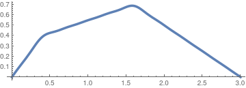
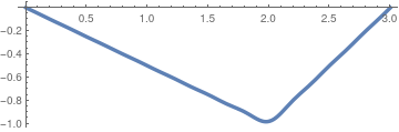
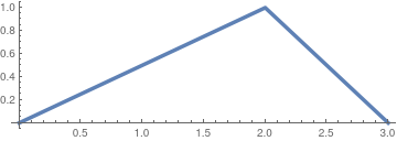
Music often involves strings that are fixed at both ends and are elastic and vibrate. The methodsin which these strings are made to vibrate, and therefore emit sound, vary across differentinstruments. In the case of a guitar, specificallyin fingerpicking, a string is plucked by pulling it upward and releasing it from rest; therefore creatinga triangular impulse shape. String vibration in strumming patterns works in a similar way, however, the strings can be forced either upward or downward by the guitar pick. Nonetheless, the initial condition consequently defines some vertical displacement, and zero vertical velocity,at t = 0. The point of which the string is plucked is usually about one third of the way down across the string.

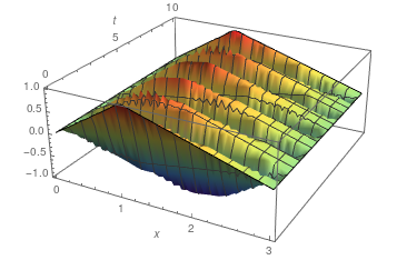
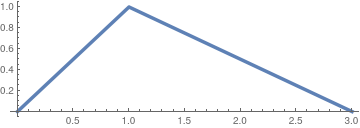
Suppose we pluck a string by pulling it upward and release it from rest (so it has a triangular form). If the point of the pluck is in the third of a string of length ℓ (which is usually the case when playing guitar), we can model the vibration of the string by solving the following initial boundary value problem:

\[ \begin{array}{ll} \ddot{u} = c^2 \,u_{xx} , & 0< x< \ell , \quad 0< t <t^{\ast} <\infty ; \\ u(0,t) = u(\ell ,t) =0, & 0<t<t^{\ast} <\infty ; \\ u(x,0^{+}) = f(x) = \begin{cases} \dfrac{3x}{\ell} , & 0 < x < \frac{\ell}{3} , \\ \dfrac{3}{2\ell} \, (\ell -x) , & \frac{\ell}{3} < x < \ell , \end{cases} \\ \dot{u} (x,0) = v(x) \equiv 0 ,\quad & 0<x< \ell . \end{array} \]
Since its solution was found previously, we get
\[ u(x,t) = \sum_{n\ge 1} A_n \cos \left( \frac{n\pi ct}{\ell} \right) \sin \left( \frac{n\pi x}{\ell} \right) , \]
where
\[ A_n = \frac{2}{\ell} \int_0^{\ell} f(x) \, \sin \left( \frac{n\pi x}{\ell} \right) {\text d} x , \qquad n=1,2,\ldots . \]
Using Mathematic, we obtain the values of coefficients An:
f[x_] = Piecewise[{{3*x/a, 0 < x < a/3}, {3/2/a*(a - x), a/3 < x < a}}];
Simplify[Assuming[Element[n, Integers] && Element[a, Reals], 2/a*Integrate[f[x]*Sin[n*Pi*x/a], {x, 0, a}]]]
\[ A_n = \frac{9}{n^2 \pi^2} \,\sin \left( \frac{n\pi}{3} \right) , \qquad n=1,2,\ldots . \]
Therefore, the solution is represented by the infinte series:
\[ u(x,t) = \sum_{n\ge 1} \frac{9}{n^2 \pi^2} \,\sin \left( \frac{n\pi}{3} \right) \cos \left( \frac{n\pi ct}{\ell} \right) \sin \left( \frac{n\pi x}{\ell} \right) . \]
Its coefficients decrease as n−2, so we plot its truncated version.
     
S20[x_, t_] = Sum[9/n^2/Pi^2*Sin[n*Pi/3]*Cos[n*Pi*t]*Sin[n*Pi*x/3], {n, 1, 20}];
Plot3D[S20[x, t], {x, 0, 3}, {t, 0, 10}, ColorFunction -> "Rainbow", AxesLabel -> Automatic]
       Solution plot            Mathematica code

We plot the solution profile at several time values.
Plot[f[x] /. a -> 3, {x, 0, 3}, PlotStyle -> Thickness[0.01], AspectRatio -> 1/3]
and then
Plot[S20[x, 0.2], {x, 0, 3}, PlotStyle -> Thickness[0.01], AspectRatio -> 1/3] Plot[S20[x, 0.4], {x, 0, 3}, PlotStyle -> Thickness[0.01], AspectRatio -> 1/3] Plot[S20[x, 0.6], {x, 0, 3}, PlotStyle -> Thickness[0.01], AspectRatio -> 1/3] Plot[S20[x, 0.8], {x, 0, 3}, PlotStyle -> Thickness[0.01], AspectRatio -> 1/3] Plot[S20[x, 1.0], {x, 0, 3}, PlotStyle -> Thickness[0.01], AspectRatio -> 1/3]
                             
       Solution at t = 0              Solution at t = 0.2              Solution at t = 0.4              Solution at t = 0.6              Solution at t = 0.8              Solution at t = 1.0

For another initial condition specified by a string having a similar triangular form (see figure below)
     
g[x_] = Piecewise[{{3*x/2/a, 0 < x < 2*a/3}, {3/a*(a - x), 2*a/3 < x < a}}];
Plot[g[x] /. a -> 3, {x, 0, 3}, PlotStyle -> Thickness[0.01], AspectRatio -> 1/3]
\[ u(x,0) = g(x) = \begin{cases} \dfrac{3x}{2\ell} , & 0 < x < \frac{2\ell}{3} , \\ \dfrac{3}{\ell} \, (\ell -x) , & \frac{2\ell}{3} < x < \ell , \end{cases} \]
the solution becomes
g[x_] = Piecewise[{{3*x/2/a, 0 < x < 2*a/3}, {3/a*(a - x), 2*a/3 < x < a}}];
Simplify[Assuming[Element[n, Integers] && Element[a, Reals], 2/a*Integrate[g[x]*Sin[n*Pi*x/a], {x, 0, a}]]]
\[ u(x,t) = \sum_{n\ge 1} \frac{9}{n^2 \pi^2} \,\sin \left( \frac{2n\pi}{3} \right) \cos \left( \frac{n\pi ct}{\ell} \right) \sin \left( \frac{n\pi x}{\ell} \right) . \]
   ■
Example 3: 
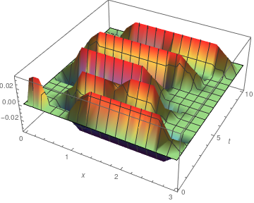
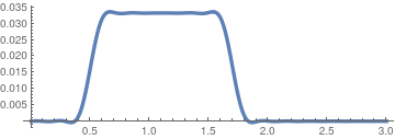
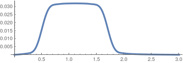
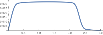
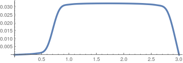
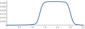
Contrary to the guitar string case, a piano involves no initial displacement. Rather, an initial velocity is created by a felt-covered hammer, which strikes the piano string when the pianist presses on a key. This velocity can be small or large,depending on how hard the key is pressed.A harder strike will cause a louder sound, and vice-versa. These piano strings can be arranged in two ways: vertically or horizontally---for upright or grand pianos, respectively. Therefore, a vertical or horizontal velocity at t = 0 is created by the hammer system, and subsequently creates sound.

Sounds from a piano, unlike the guitar, are put into effect by striking strings. When a player presses a key, it causes a hammer to strike the strings. The corresponding IBVP is

\begin{equation*} \begin{split} &\text{(PDE, partial differential equation)} \quad u_{tt} = c^2 u_{xx} , \quad 0<x<\ell, \ 0< t\le t^{\ast} < \infty , \\ &\text{(BC, boundary conditions)} \hspace{6.2mm} u(0,t) =0 , \quad u (\ell ,t) =0 , \quad 0< t\le t^{\ast} < \infty , \\ &\text{(IC, initial conditions)} \qquad u(x,0) =0 , \quad u_t (x,0) = v(x) , \end{split} \end{equation*}
where the initial velocity is the step function
\[ v(x) = \begin{cases} 1 , & \mbox{ when } s< x< s+h , \\ 0, & \mbox{ otherwise. } \end{cases} \]
Here s is a position of the left hammer's end and h is the width of the hammer. It is assumed that both s and s+h are within the string length ℓ.

Since the boundary conditions are homogeneous, we can apply the separation of variables method. According to this method, we seek partial nontrivial (= not identically zero) solutions of the wave equation satisfying the homogeneous boundary conditions and representing as a product of two functions: \( u(x,t) = X(x)\,T(t) . \) Substituting this function into the wave equation gives

\[ \frac{X''(x)}{X(x)} = \frac{\ddot{T}(t)}{c^2 T(t)} = -\lambda . \]
Separation of variables yields
\[ \begin{split} \ddot{T}(t) + c^2 \lambda\, T(t) &=0 , \\ X'' (x) + \lambda \,X(x) &=0 . \end{split} \]
Similarly to the previous sections, we substitute \( u(x,t) = X(x)\,T(t) \) into the boundary conditions to obtain X(0) = 0 and X(ℓ) = 0. The differential equation together with these boundary conditions constitute the Sturm--Liouville problem:
\[ X'' (x) + \lambda \,X(x) =0, \qquad X(0) =0, \quad X(\ell ) =0 . \]
Of the usual three possibilities for the parameter, λ = 0, λ = -α² < 0, and λ = α² > 0, only the last choice leads to nontrivial solutions. Corresponding to λ = α² > 0, with α > 0, the general solution to the differential equation \( X'' (x) + \alpha^2 \,X(x) =0 \) is
\[ X(x) = c_1 \cos \alpha x + c_2 \sin \alpha x . \]
The boundary conditions X(0) = 0 and X(ℓ) = 0 dictate that c1 = 0 and \( c_2 \sin \alpha \ell =0 . \) The last equation implies that \( \sin \alpha \ell =0 \) because otherwise c2 = 0 forces to obtain a trivial solution. Since we cannot effort vanishing c2, we have to choose α to be
\[ \alpha = \sqrt{\lambda} = \frac{n\pi}{\ell} , \qquad n=1,2,3,\ldots . \]
Therefore, we obtain the eigenvalues and corresponding eigenfunctions:
\[ \lambda_n = \left( \frac{n\pi}{\ell} \right)^2 , \qquad X_n (x) = \sin \frac{n\pi x}{\ell}, \qquad n=1,2,3,\ldots . \]
The general solution of the second order differential equation \( \ddot{T} + c^2 \lambda_n T(t) =0 \) becomes
\[ T_n (t) = A_n \cos \frac{cn\pi t}{\ell} + B_n \sin \frac{cn\pi t}{\ell} , \qquad n=1,2,3,\ldots . \]
Finally, we represent the required solution of the given initial boundary value problem as the sum of all partial nontrivial solutions
\[ u(x,t) = \sum_{n\ge 1} u_n (x,t) = \sum_{n\ge 1} X_n (x) \, T_n (t) = \sum_{n\ge 1} \sin \frac{n\pi x}{\ell} \left( A_n \cos \frac{cn\pi t}{\ell} + B_n \sin \frac{cn\pi t}{\ell} \right) . \]
Setting t = 0, we get from the initial condition u(x,0) = 0 that yields
\[ u(x,0) = 0 = \sum_{n\ge 1} u_n (x,0) = \sum_{n\ge 1} A_n X_n (x) = \sum_{n\ge 1} A_n \sin \frac{n\pi x}{\ell} . \]
Therefore, all coefficients An are zeroes. From the second initial condition, we get
\[ u_t (x,0) = v(x) = \sum_{n\ge 1} T'_n (0)\, X_n (x) = \sum_{n\ge 1} \frac{cn\pi}{\ell} \,B_n \sin \frac{n\pi x}{\ell} . \]
Since this is just the sine Fourier series for function v(x), we immediately find its coefficients:
\[ B_n = \frac{2}{cn\pi} \int_0^{\ell} v(x)\, \sin \frac{n\pi x}{\ell} \,{\text d}x . \]
Using the given form of the initial velocity, we obtain
\[ B_n = \frac{2}{cn\pi} \int_s^{s+h} \sin \frac{n\pi x}{\ell} \,{\text d}x = \frac{2\ell}{cn^2 \pi^2} \left[ \cos \frac{n\pi s}{\ell} - \cos \frac{n\pi (s+h)}{\ell} \right] . \]
2/(c*n*Pi) *Integrate[Sin[n*Pi*x/L], {x, s, s + h}]
(2 L (Cos[(n \[Pi] s)/L] - Cos[(n \[Pi] (h + s))/L]))/(c n^2 \[Pi]^2)
Substituting these values of coefficients Bn into the general formula, we arrive at the required solution
\[ u(x,t) = \sum_{n\ge 1} \frac{2\ell}{cn^2 \pi^2} \left[ \cos \frac{n\pi s}{\ell} - \cos \frac{n\pi (s+h)}{\ell} \right] \sin \frac{n\pi x}{\ell} \, \sin \frac{cn\pi t}{\ell} . \]
      We plot the solution function with 30 terms and s = 1.0,h = 0.2:
s = 1.0; h = 0.2;
P30[x_, t_] = Sum[2/n^2/Pi^2 *(Cos[n*Pi*s/3] - Cos[n*Pi*(s + h)/3])*Sin[n*Pi*x/3]* Sin[n*Pi*t], {n, 1, 30}];
Plot3D[P30[x, t], {x, 0, 3}, {t, 0, 10}, ColorFunction -> "Rainbow", AxesLabel -> Automatic]
       Solution plot            Mathematica code

To clarify the wave oscillations, we plot the solution at some grid of time variables.
Plot[P30[x, 0.2], {x, 0, 3}, PlotStyle -> Thickness[0.01], AspectRatio -> 1/3]
Plot[P30[x, 0.4], {x, 0, 3}, PlotStyle -> Thickness[0.01], AspectRatio -> 1/3]
Plot[P30[x, 0.6], {x, 0, 3}, PlotStyle -> Thickness[0.01], AspectRatio -> 1/3]
Plot[P30[x, 0.8], {x, 0, 3}, PlotStyle -> Thickness[0.01], AspectRatio -> 1/3]
Plot[P30[x, 1.2], {x, 0, 3}, PlotStyle -> Thickness[0.01], AspectRatio -> 1/3]
                       
       Solution at t = 0.2              Solution at t = 0.4              Solution at t = 0.6              Solution at t = 0.8              Solution at t = 1.2

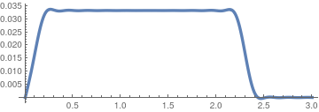
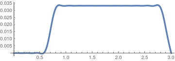
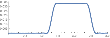
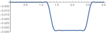
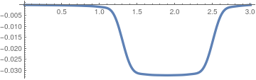
Since the input function is piecewise continuous, its approximations clearly show the Gibbs phenomena. To eliminate it, we apply the Cesàro summation procedure.
C30[x_, t_] = Sum[2/n^2/Pi^2 *(Cos[n*Pi*s/3] - Cos[n*Pi*(s + h)/3])*Sin[n*Pi*x/3]* Sin[n*Pi*t]*(1 - n/30), {n, 1, 30}];
Plot[C30[x, 0.2], {x, 0, 3}, PlotStyle -> Thickness[0.01], AspectRatio -> 1/3]
Plot[C30[x, 0.4], {x, 0, 3}, PlotStyle -> Thickness[0.01], AspectRatio -> 1/3]
Plot[C30[x, 0.6], {x, 0, 3}, PlotStyle -> Thickness[0.01], AspectRatio -> 1/3]
Plot[C30[x, 0.8], {x, 0, 3}, PlotStyle -> Thickness[0.01], AspectRatio -> 1/3]
Plot[C30[x, 1.2], {x, 0, 3}, PlotStyle -> Thickness[0.01], AspectRatio -> 1/3]
                       
       Cesàro solution at t = 0.2              Cesàro solution at t = 0.4              Cesàro solution at t = 0.6              Cesàro solution at t = 0.8              Cesàro solution at t = 1.2

   ■
Example 4: Helmholtz was the first to study systematically the physics of violin strings and his results are covered in Tonempfind-ungen, his groundbreaking treatise on the scientific theory of music. The key point is that the friction between the bow and the violin string varies with the relative velocity between them. When the relative velocity is zero or small, the friction is large. As the relative velocity increases, the friction decreases. Rosin (also called colophony or Greek pitch) is applied to the horsehairs in the violin bow to maximize this velocity dependence of the friction withthe string.The frictional force exerted by the bow on the string is therefore modulated in phase with the string’s velocity,allowing the bow to do net work over a complete period of the string’s oscillation (see Eq. (6)). Thus, as the bow isdrawn over the violin string, a negative damping is obtained and the resonant vibration grows exponentially, until itreaches a limiting, nonlinear “stick-slip” regime.

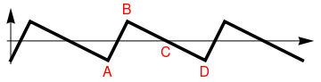
As Helmholtz observed experimentally, in this nonlinear stick-slip regime the waveform for the displacement of the violin string is triangular. First, the violin string sticks to the bow and moves at the same velocity at which the bow is being drawn. This is represented in Fig. 6 by the motion between Aand B. At B the string unsticks and moves back to equilibrium, which it passes at C. It continues moving with nearly the same velocity until at D it again becomes stuck to the bow. Between A and B the frictional force exerted by the bow on the string is positive and large, while between B and D the frictional force is still positive but small. Figure 6 also shows that if the bow is drawn faster,the string plays the same note, but with a greater amplitude. Within certain limits, the amplitude of the vibration is proportional to the speed of the bow.

      Waveform for the displacement u(t) of a violin string in the limiting “stick-slip” regime, as first measured by Helmholtz. Between A and B the string moves with the bow, while between B and D it moves against the bow.
line = Graphics[{{Thickness[.01], Line[{{0, -1}, {1, 1}, {5, -1}, {6, 1}, {10, -1}, {11, 1}, {15, -1}}]}}]
ax = Graphics[{Arrowheads[0.05], Arrow[{{-0.2, 0}, {15.6, 0}}]}];
ay = Graphics[{Arrowheads[0.05], Arrow[{{0, -1.2}, {0, 1.7}}]}];
tA = Graphics[Text[Style["A", FontSize -> 16, Red], {5, -1.6}]];
tB = Graphics[Text[Style["B", FontSize -> 16, Red], {6, 1.6}]];
tC = Graphics[Text[Style["C", FontSize -> 16, Red], {8, -0.6}]];
tD = Graphics[Text[Style["D", FontSize -> 16, Red], {10, -1.6}]];
Show[line, ax, ay, tA, tB, tC, tD]
       Waveform for the displacement of violin string.            Mathematica code

   ■


Justification of the Solution


Note that \( a_0 = u(x,t) . \)


Dispersive Waves


Consider the modified wave equation
\[ u_{tt} = c^{-2} u_{tt} + \gamma^2 u \]
with the homogeneous Dirichlet conditions u(0, t) = u(ℓ, t) = 0 and the guitar initial conditions. Its solution can be represented as an infinite series
\[ u(x,t) = \sum_{n\ge 1} c_n \cos \left( \sqrt{\frac{n^2 \pi^2}{\ell^2} + \gamma^2} \,ct \right) \sin \frac{n\pi x}{\ell} , \]
where
\[ c_n = \frac{2}{\ell} \int_0^{\ell} u(x,0)\,\sin \frac{n\pi x}{\ell} \,{\text d}x , \qquad n=1,2,3,\ldots . \]
Using the trigonometric identity
\[ 2\,\sin\alpha\, \cos\beta = \sin \left( \alpha + \beta \right) + \sin \left( \alpha - \beta \right) , \]
we transfer the formula to the following one:
\[ u(x,t) = \frac{1}{2} \sum_{n\ge 1} c_n \left[ \sin \frac{n\pi}{\ell} \left( x + a_n t \right) + \sin \frac{n\pi}{\ell} \left( x - a_n t \right) \right] , \]
where
\[ a_n = \left( \frac{n\pi}{\ell} \right)^{-1} \sqrt{\frac{n^2 \pi^2}{\ell^2} + \gamma^2} \,c . \]
﹡ ⁎ ✱ ✲ ✳ ✺ ✻ ✼ ✽ ❋


Consider another modified wave equation subject to the damping force
\[ u_{tt} = c^{-2} u_{tt} -2k\, u_t , \]
with the same initial and boundary conditions as in the previous subsection.

Separation of variables u(x, t) = X(x)T(t) yields the Sturm--Liouville problem for X(x)

\[ X'' (x) + \lambda\, X(x) = 0, \qquad X(0) = 0, \quad X(\ell ) = 0, \]
and the differential equation for T(t):
\[ T'' (t) + 2k\, T' (t) + \lambda\,c^2 T(t) = 0 . \]
We know how to solve the Sturm--Liouville problem:
\[ \lambda_n = \left( \frac{n\pi}{\ell} \right)^2 , \qquad X_n = \sin \left( \frac{n\pi x}{\ell} \right) , \qquad n= 1,2, 3 \ldots . \]
To find the solution for T(t), we substitute \( T(t) = e^{rt} \) into the differential equation and obtain the quadratic equation for r:
\[ r^2 + 2k\,r + \lambda_n c^2 = 0. \]
Solving this quadratic equation for r gives
\[ r = -k \pm \sqrt{k^2 - c^2 \lambda_n} \]
The solution Tn(t) corresponding to the eigenvalues λ = λn are all oscillatory if r has a complex part, i.e. if k² < c²λn for all n, or
\[ k^2 < \min_{n\ge 1} c^2 \lambda_n = \min_{n\ge 1} \left( \frac{cn\pi}{\ell} \right)^2 \]
This gives the criterion that all the Tn(t) be oscillatory
\[ 0 \ge k < \frac{c\pi}{\ell} . \]
The solution Tn(t) is a linear combination of exp(rt):
\[ T_n (t) = a_n e^{-kt + t{\bf j}\sqrt{c^2 \lambda^2_n - k^2}} + b_n e^{-kt - t{\bf j}\sqrt{c^2 \lambda^2_n - k^2}} \]
or, upon extracting the real parts,
\[ T_n (t) = e^{-kt} \left( a_n \cos t\sqrt{c^2 \lambda^2_n - k^2} + b_n \sin t\sqrt{c^2 \lambda^2_n - k^2} \right) . \]
The corresponding modes are
\[ u_n (x,t) = X_n (x)\,T_n (t) = e^{-kt} \left( a_n \cos t\sqrt{c^2 \lambda^2_n - k^2} + b_n \sin t\sqrt{c^2 \lambda^2_n - k^2} \right) \sin \frac{n\pi x}{\ell} . \]
For positive damping coefficient (k > 0), the normal mode decays with time and oscillates as it decays. The corresponding frequencies of mode's oscillations is
\[ \nu_n = \frac{1}{2\pi} \,\sqrt{c^2 \lambda_n - k^2} = \frac{1}{2\pi} \,\sqrt{\frac{c^2 n^2 \pi^2}{\ell^2} - k^2} = \frac{cn}{2\ell} \sqrt{1 - \left( \frac{\ell k}{cn\pi} \right)^2} .


  1. Grigoryan, V, Partial Differential Equations, 2010, University of California, Santa Barbara.
  2. Haberman, R., Applied Partial Differential Equations with Fourier Series and Boundary Value Problems, Pearson; 5th edition, 2012. ISBN-13 : 978-0321797063
  3. Helmholtz, H., On the Sensations of Tone as a Physiological Basis for the Theory of Music, 2nd English ed., (New York: Dover, 1954),


Return to Mathematica page
Return to the main page (APMA0340)
Return to the Part 1 Matrix Algebra
Return to the Part 2 Linear Systems of Ordinary Differential Equations
Return to the Part 3 Non-linear Systems of Ordinary Differential Equations
Return to the Part 4 Numerical Methods
Return to the Part 5 Fourier Series
Return to the Part 6 Partial Differential Equations
Return to the Part 7 Special Functions