Return to computing page for the second course APMA0340
Return to Mathematica tutorial for the first course APMA0330
Return to Mathematica tutorial for the second course APMA0340
Return to the main page for the first course APMA0330
Return to the main page for the second course APMA0340
Return to Part I of the course APMA0340
Introduction to Linear Algebra with Mathematica
Glossary
Preface
This section presents some properties of the most remarkable and useful in numerical computations Chebyshev polynomials of first kind \( T_n (x) \) and second kind \( U_n (x) .\) Both Chebyshev polynomials are eigenfunctions of the corresponding singular Sturm--Liouville problems. Other two Chebyshev polynomials of the third kind and the fourth kind are not so popular in applications.
Best Approximations
A problem of finding the best approximation to a given function f(x) depends what distance between functions is in use. In a space of continuous function on an interval [𝑎, b], usually denoted by C[𝑎, b], we consider the distances generated by the norms:
- uniform norm \( \displaystyle \| f(x) \|_{\infty} = \sup_{a \lle x \le b} \left\vert f(x) \right\vert ; \)
- least squared or 𝔏² norm \( \displaystyle \| f(x) \|_{2} = \left\{ \int_a^b w(x)\,f^2 (x)\,{\text d}x \right\}^{1/2} , \) for some positive integrable function w(x), called weight;
- 𝔏¹ norm \( \displaystyle \| f(x) \|_{1} = \int_a^b \left\vert f (x)\right\vert {\text d}x . \)
It is of considerable importance to determine a such approfimation p(x) to a given function f(x) that gives
Zeroes of Chebyshev polynomials
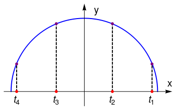
From the general theorem about zeroes of orthogonal polynomials, it follows that a Chebyshev polynomial of either kind of degree n has n different simple roots, called Chebyshev roots (or Chebyshev nodes), in the interval [−1,1]. The roots of the Chebyshev polynomial of the first kind are sometimes called Chebyshev nodes because they are used as nodes in polynomial interpolation. The extrema of Chebyshev polynomials of first kind are located at
For demonstration, we consider the Chebyshev polynomial of the first kind, T4(x) = 8x3 −8x² + 1; its nodes are
ar2 = Graphics[{Black, Arrow[{{0.0, -0.2}, {0.0, 1.2}}]}];
line1 = Graphics[{Black, Dashed, Thick, Line[{{0.924, 0}, {0.924, 0.35}}]}];
line2 = Graphics[{Black, Dashed, Thick, Line[{{0.383, 0}, {0.383, 0.92}}]}];
line3 = Graphics[{Black, Dashed, Thick, Line[{{-0.383, 0}, {-0.383, 0.92}}]}];
line4 = Graphics[{Black, Dashed, Thick, Line[{{-0.924, 0}, {-0.924, 0.35}}]}];
dx1 = Graphics[{Red, Disk[{0.924, 0}, 0.02]}];
dx4 = Graphics[{Red, Disk[{-0.924, 0}, 0.02]}];
dx3 = Graphics[{Red, Disk[{-0.383, 0}, 0.02]}];
dx2 = Graphics[{Red, Disk[{0.383, 0}, 0.02]}];
dy1 = Graphics[{Purple, Disk[{0.924, 0.376}, 0.02]}];
dy4 = Graphics[{Purple, Disk[{-0.924, 0.376}, 0.02]}];
dy2 = Graphics[{Purple, Disk[{0.383, 0.926}, 0.02]}];
dy3 = Graphics[{Purple, Disk[{-0.383, 0.926}, 0.02]}];
txt1 = Graphics[Text[Style[Subscript[t, 1], 20], {0.92, -0.11}]];
txt2 = Graphics[Text[Style[Subscript[t, 2], 20], {0.383, -0.11}]];
txt3 = Graphics[Text[Style[Subscript[t, 2], 20], {-0.383, -0.11}]];
txt4 = Graphics[Text[Style[Subscript[t, 4], 20], {-0.92, -0.11}]];
tx = Graphics[Text[Style["x", 20], {1.17, 0.11}]];
ty = Graphics[Text[Style["y", 20], {0.17, 1.11}]];
Show[circle, ar1, ar2, line1, line2, line3, line4, dx1, dx2, dx3, dx4, dy1, dy2, dy3, dy4, txt1, txt2, txt3, txt4, tx, ty]
Since the total number of extreme nodes xk is n + 1, the derivative of the Chebyshev polynomial of the first kind Tn(x) on interval (−1, 1) has n −1 zeroes. Hence the Chebyshev polynomial outside the closed interval [−1, 1] is monotonic. Therefore, all oscillations occur within interval [−1, 1] and \( \left\vert T_n (x) \right\vert &le 1 . \) Moreover
- Clenshaw, C.W., Norton, H.J.: The solution of nonlinear ordinary differential equations in chebyshev series. The Computer Journal, 1963, {\bf 6}, Issue 1, 88–92; https://doi.org/10.1093
Return to Mathematica page
Return to the main page (APMA0340)
Return to the Part 1 Matrix Algebra
Return to the Part 2 Linear Systems of Ordinary Differential Equations
Return to the Part 3 Non-linear Systems of Ordinary Differential Equations
Return to the Part 4 Numerical Methods
Return to the Part 5 Fourier Series
Return to the Part 6 Partial Differential Equations
Return to the Part 7 Special Functions