Preface
The Lambert special function is the topic of this section.
Return to computing page for the second course APMA0340
Return to Mathematica tutorial for the first course APMA0330
Return to Mathematica tutorial for the second course APMA0340
Return to the main page for the first course APMA0330
Return to the main page for the second course APMA0340
Return to Part VII of the course APMA0340
Introduction to Linear Algebra with Mathematica
Glossary
Lambert Functions
The Lambert W function, also called the omega function or product logarithm, is a set of branches of the inverse relation of the function \( f(z) = z\, e^z , \) where ez is the exponential function, and z is any complex number. In other words

The function W is called after the Swiss polymath Johann Heinrich Lambert (1728--1777) who found in 1758 series representation of the root for the equation \( y = q + y^m . \) Later his long time friend Leonhard Euler (1707--1783) solve more symmetric equation \( y^{\alpha} - y^{\beta} = \nu \left( \alpha - \beta \right) y^{\alpha + \beta} . \) Lambert is credited with the first proof that π is irrational by using a generalized continued fraction for the function tan x. He was the first mathematician to address the general properties of map projections. Lambert invented the first practical hygrometer.
Many years later in 1980th, a group of scientists (Gaston H. Gonnet, Robert M. Corless, Donald Knuth, and David Jeffrey) used the Lambert function in their research; shortly Donald Knuth from Stanford University suggested to call it the Lambert W function.
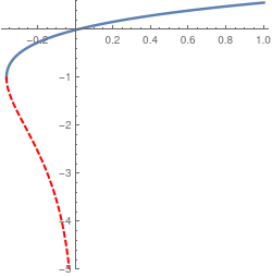
The Lambert W function in neither odd nor even. It is defined on the interval \( \left( - e^{-1}, \infty \right) \) and range from minus infinity to plus infinity. There are countably many branches of the W function, denoted by Wk(z), for integer k∈ℤ. A point A with coordinates \( \left( - e^{-1}, -1 \right) \) divides the graph into two branches that share the same vertical tangent line. The upper branch, usually denoted as W0, is called the main (or principal) branch because it goes through the origin. The lower branch W-1 has the inflection point at \( \left( - 2\,e^{-2}, -2 \right) \) and vertical asymptote at x = 0.
In general, for a given complex z, the defining equation will have an infinite number of solutions and is therefore a multivalued analytic function. Its principal branch is denoted by W0(z); other branches are labeled with Wk(z), k ∈ ℤ. However, only two of them are real-valued functions that correspond k = 0 and k = −1. So one real solution of the defining Lambert equation is W0(x) or simply W(x) for −1/e ≤ x < ∞, while the secondary real branch satisfying W(x) ≤ −1 is denoted by W-1(x), −1/e ≤ x < 0.
Mathematica has a special command to evaluate and plot the Lambert W function: ProductLog[x] for the principal branch and ProductLog[k, x] for k-th branch.

Gaston Gonnet, Rob Corless, Don Knuth, and David Jeffrey.
|
Now we plot the Lambert principal branch W0(x) and the next to it branch W-1(x).
k0 = Plot[ProductLog[x], {x, -1/E, 1}, PlotStyle -> Thickness[0.01],
PlotRange -> {-5, 0.6}];
km1 = Plot[ProductLog[-1, x], {x, -1/E, -0.01}, PlotStyle -> {Thick, Red, Dashed}, PlotRange -> {-5, 0.6}]; Show[k0, km1, AspectRatio -> 1] |
|
| Plots of the principal branch (in blue) and W-1 in red. | Mathematica code |
For other indices k ≠ 0, -1, the branches Wk of the Lambert function are complex-valued. The following identities follow from the definition:
The Lambert function has many applications that are documented in the reference sources.
Example: Consider an RC-circuit having a resistance linearly proportional to the temperature:
In dimensionless variables, the above system becomes
To solve the above system of differential equations, we introduce a new variable
Example: Let a=<1,3,-4> and b=<-1,1,-2> be two vectors. Find \( {\bf a}\cdot ({\bf a}\times {\bf b}), \) where \( {\bf a}\cdot {\bf b} \) is dot product, and \( {\bf a}\times {\bf b} \) is cross product of two vectors. Input variables are vecors a and b. Function will calculate the cross product of a and b, and then calculate the dot product of that value and a. Notice that any input values for a and b will result in zero sum.
b={-1,1,-2}
c=a.Cross[a,b]
{-1,1,-2}
0
- Corless, R.M., Gonnet, G.H., Hare, D.E.G., Jeffrey, D.J., and Knuth, D.E., (1996). "On the Lambert W function," Advances in Computational Mathematics, 1996, Vol. 5: pp. 329–359. doi:10.1007/BF02124750
- Dobrushkin, V.A., Methods in Algorithmic Analysis, CRC Press, Boca Raton, 2010.
- Dubinov, A.E., Dubinova, I.D., and Saǐkov, S.K., (2006). The Lambert W Function and Its Applications to Mathematical Problems of Physics (in Russian). RFNC-VNIIEF. Sarov, Russia. 169p.
- Jeffrey, D.J., Hare, D.E.G., and Corless, R.M., Unwinding the branches of the Lambert W function, The Mathematical Scientist, 1966, Vol. 21, No. 1, p. 1--2.
- Lambert, J.H., Observationes variae in mathesin puram, Acta Helveticae physico-mathematico-anatomico-botanico-medica, Band III, 128–168, 1758. http://www.kuttaka.org/~JHL/L1758c.pdf
- Ontario Research Centre for Computer Algebra, 2004. The Lambert W function—Poster. Available from: http://www.orcca.on.ca/LambertW/
- Parker, F.D., Integrals of inverse functions, American Mathematical Monthly, 1955, Vol. 62, No. 6, 439--440.
- Valluri, S.R., Jeffrey, D.J., and Corless, R.M., Some applications of the Lambert W function to physics, Canadian Journal of Physics, Vol. 78, 823--831, 2000.
- https://en.wikipedia.org/wiki/Lambert_W_function
Return to Mathematica page
Return to the main page (APMA0340)
Return to the Part 1 Matrix Algebra
Return to the Part 2 Linear Systems of Ordinary Differential Equations
Return to the Part 3 Non-linear Systems of Ordinary Differential Equations
Return to the Part 4 Numerical Methods
Return to the Part 5 Fourier Series
Return to the Part 6 Partial Differential Equations
Return to the Part 7 Special Functions