In applications, people deal with a variety of quantities that are used to describe the physical world. Examples of
such quantities include distance, displacement, speed, velocity, acceleration, force, mass, momentum, energy, work,
power, etc. All these quantities can by divided into two categories -- vectors and scalars. A vector quantity is a
quantity that is fully described by both magnitude and direction. On the other hand, a scalar quantity is a quantity
that is fully described by its magnitude.
In mathematics, physics, and engineering, a Euclidean vector
(simply a vector) is a geometric object that has magnitude (or length) and
direction. Many familiar physical notions, such as forces, velocities, and
accelerations, involve both magnitude (the amount of the force, velocity, or
acceleration) and a direction. In most physical situations involving vectors,
only the magnitude and direction of the vector are significant; consequently,
we regard vectors with the same length and direction as being equal
irrespective to their positions.
It is a custom to identify vectors with arrows (geometric object). The tail of
the arrow is called the initial point of the vector and the
tip the terminal point. To emphasis this approach, an arrow
is placed above the initial and terminal points, for example, the notation
\( {\bf v} = \vec{AB} \) tells us that A is
the starting point of the vector v and its terminal point is
B. In this tutorial (as in most science papers and textbooks), we will
denote vectors in boldface type applied to lower case letters such as
v, u, or x.
Any two vectors x and y can be added in "tail-to-head" manner; that is, either
x or y may be applied to any point and then another vector is applied to the
endpoint of the first. If this is done, the endpoint of the latter is the endpoint of their sum, which is denoted
by x + y. Besides the operation of vector addition there is another natural
operation that can be performed on vectors---multiplication by a scalar that are often taken to be real numbers.
When a vector is multiplied by a real number k, its magnitude is multiplied by |k| and its direction
remains the same when k is positive and the opposite direction when k is negative. Such vector is
denoted by kx.
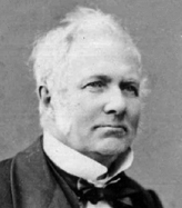
The concept of vector, as we know it today, evolved gradually over a period of more than 200 years. The Italian
mathematician, senator, and municipal councilor Giusto Bellavitis (1803--1880) abstracted the basic idea in 1835.
The idea of an n-dimensional Euclidean space for n > 3 appeared in a work on the divergence theorem
by the Russian mathematician Michail Ostrogradsky (1801--1862) in 1836, in the geometrical tracts of Hermann Grassmann (1809--1877) in the early 1840s,
and in a brief paper of Arthur Cayley (1821--1895) in 1846. Unfortunately, the first two authors were virtually ignored in their lifetimes.
In particular, the work of Grassmann was quite philosophical and extremely difficult to read.
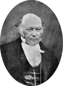
The term vector was introduced by the Irish mathematician, astronomer, and mathematical physicist William Rowan
Hamilton (1805--1865) as part of a quaternion.
Vectors can be described also algebraically. Historically, the first vectors were Euclidean vectors that can be
expanded through standard basic vectors that are used as coordinates. Then any vector can be uniquely represented
by a sequence of scalars called coordinates or components. The set of such ordered n-tuples is denoted by
\( \mathbb{R}^n . \) When scalars are complex numbers, the set of ordered n-tuples
of complex numbers is denoted by \( \mathbb{C}^n . \) Motivated by these two approaches, we
present the general definition of vectors.
A vector spaceV over set of either real numbers or complex numbers is a set of elements,
called vectors, together with two operations that satisfy the eight axioms listed below.
1. The first operation is an inner operation that assigns to any two vectors x and y
a third vector which is commonly written as x + y and called the sum of these two
vectors.
2. The second operation, is an outer operation that assigns to any scalar k and vector x another vector,
denoted by kx.
Commutativity of addition: \( ({\bf v} + {\bf u}) = {\bf u} + {\bf v} \)
for \( ({\bf v} , {\bf u}) \in V . \)
Identity element of addition: there exists an element \( ({\bf 0} \in V , \) called
the zero vector, such that \( {\bf v} +{\bf 0}) = {\bf v} \) for every vector from V.
Inverse elements of addition: for every vector v, there exists an element
\( -{\bf v} \in V , \) called the additive inverse of v, such that
\( {\bf v} + (-{\bf v}) = {\bf 0} . \)
Compatibility of scalar multiplication with field multiplication: \( a(b{\bf v}) = (ab){\bf v} \)
for any scalars a and b and arbitrary vector v.
Identity element of scalar multiplication: \( 1{\bf v} = {\bf v} , \) where 1
denotes the multiplicative identity.
Distributivity of scalar multiplication with respect to vector addition: \( k\left( {\bf v} +
{\bf u}\right) = k{\bf v} + k{\bf u} \) for any scalar k and arbitrary vectors v and u.
Distributivity of scalar multiplication with respect to field addition: \( \left( a+b \right)
{\bf v} = a\,{\bf v} + b\,{\bf v} \) for any two scalars a and b and arbitrary vector v.
■
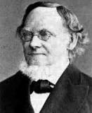
Hermann Grassmann
Historically, the first ideas leading to vector spaces can be traced back as far as the 17th century;
however, the idea crystallized with the work of the Prussian/German mathematician Hermann Günther Grassmann (1809--1877), who
published a paper in 1862. He was also a linguist, physicist, neohumanist, general scholar, and publisher.
His mathematical work was little noted until he was in his sixties. It is interested that while he was a student
at the University of Berlin, Hermann studied theology, also taking classes in classical languages, philosophy, and
literature. He does not appear to have taken courses in mathematics or physics. Although lacking university training
in mathematics, it was the field that most interested him when he returned to Stettin (Province of Pomerania,
Kingdom of Prussia; present-day Szczecin, Poland) in 1830 after completing his studies in Berlin.
Example: The set \( \mathbb{R}^n \mbox{ or } \mathbb{C}^n \) of all ordered n-tuples of real or complex numbers
is our first familiar example of vector spaces. This space has a standard basis: \( {\bf e}_1 =
(1,0,0,\ldots ,0 ) ,\quad {\bf e}_2 = (0,1,0,\ldots , 0 ), \ldots , {\bf e}_n = (0,0,\ldots , 0,1) .\)
In ℝ³ these unit vectors are denoted by
The above representation v = (v1,
v2, ... ,vn) of vectors in
ℝn is called the comma-delimited form. However, since
a vector in ℝn is just a list of its n components in a
specific order, any notation that displays those components in the correct
order is a valid way of representing the vector. For example, the vector can
be written as
Mathematica does not distinguish
columns from rows, so the user should specify which object is in use. A string is a grouping or ordering collection of
characters or symbols with quotes around them such as S = "Mary had a little lamb".
In Mathematica, there are no sets since Mathematica requires that an ordering be placed on its data,
and so it deals with lists that can be treated as sets if you ignore the order of the elements in the lists.
The list of elements a, b, and c is embraced into curly brackets as
L= { a, b, c } which Mathematica considers as a row-vector. The empty list is { }, and L[[k]] is the
k-th element of list L.
Let us define two vectors, one as a row denoted v1, and another as a column denoted v2:
v1 = { 1, 2, 3}
v2 = {{1}, {2}, {3}}
We can also check that they are row vector and column vector, respectively, with the command:
v1 // TraditionalForm
v2 // MatrixForm
So v1 is a 1×3 matrix; while v2 would be column vector, which is
a 3×1 matrix. Therefore, these two vectors have different dimensions and
cannot be added. Nevertheless, Mathematica does not care and if one
enter
v1 + v2
the output will be the 3-column vector:
{ {2}, {4}, {6} }
Example: Set of continuous functions. Let |a,b| denote an open or closed
or semiclosed interval on the real axis. The set \( C(|a,b|) \) of all continuous functions
on the interval |a,b| is a vector space.
Example: A polynomial of degree n is an expression of the form
where n is a nonnegative integer and each coefficient ai is a scalar/number. The zero
polynomial is the polynomial having all coefficients to be zero. The polynomials \( p_n (x) =
a_0 + a_1 x + \cdots + a_n x^n \) and \( q_n (x) =
b_0 + b_1 x + \cdots + b_m x^m \) , where for simplicity \( n\ge m , \) can be added:
Under these operations of addition and scalar multiplication, the set of all polynomials of degree not exceeding
n is a vector space.
The dot product of two vectors of the same size
\( {\bf x} = \left[ x_1 , x_2 , \ldots , x_n \right] \) and
\( {\bf y} = \left[ y_1 , y_2 , \ldots , y_n \right] \) (independently whether they are columns or rows) is the number,
denoted either by \( {\bf x} \cdot {\bf y} \) or \( \left\langle {\bf x} , {\bf y} \right\rangle ,\)
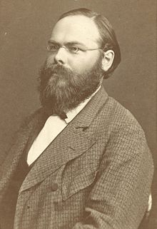
Josiah Gibbs
The dot product was first introduced by the American physicist and mathematician Josiah Willard Gibbs (1839--1903) in the 1880s.
An outer product is the tensor product of two coordinate vectors \( {\bf u} = \left[ u_1 , u_2 , \ldots , u_m \right] \) and
\( {\bf v} = \left[ v_1 , v_2 , \ldots , v_n \right] , \) denoted \( {\bf u} \otimes {\bf v} , \) is
an m-by-n matrix W such that its coordinates satisfy \( w_{i,j} = u_i v_j . \)
The outer product \( {\bf u} \otimes {\bf v} , \) is equivalent to a matrix multiplication
\( {\bf u} \, {\bf v}^{\ast} , \) (or \( {\bf u} \, {\bf v}^{\mathrm T} , \) if vectors are real) provided that u is represented as a
column \( m \times 1 \) vector, and v as a column \( n \times 1 \) vector. Here \( {\bf v}^{\ast} = \overline{{\bf v}^{\mathrm T}} . \)
For three dimensional vectors \( {\bf a} = a_1 \,{\bf i} + a_2 \,{\bf j} + a_3 \,{\bf k} =
\left[ a_1 , a_2 , a_3 \right] \) and
\( {\bf b} = b_1 \,{\bf i} + b_2 \,{\bf j} + b_3 \,{\bf k} = \left[ b_1 , b_2 , b_3 \right] \) , it is possible to define special multiplication, called cross-product:
In Mathematica, the outer product has a special command:
Outer[Times, {1, 2, 3, 4}, {a, b, c}]
Out[1]= {{a, b, c}, {2 a, 2 b, 2 c}, {3 a, 3 b, 3 c}, {4 a, 4 b, 4 c}}
An inner product of two vectors of the same size, usually denoted by \( \left\langle {\bf x} , {\bf y} \right\rangle ,\) is a generalization of the dot product if it satisfies the following properties:
\( \left\langle {\bf v} , {\bf v} \right\rangle \ge 0 , \) and equal if and only if
\( {\bf v} = {\bf 0} . \)
The fourth condition in the list above is known as the positive-definite condition.
A vector space together with the inner product is called an inner product space. Every inner product space is a metric space. The metric or norm is given by
The nonzero vectors u and v of the same size are orthogonal (or perpendicular) when their inner product is zero:
\( \left\langle {\bf u} , {\bf v} \right\rangle = 0 . \) We abbreviate it as \( {\bf u} \perp {\bf v} . \)
A generalized length function on a vector space can be imposed in many different ways, not necessarily through the
inner product. What is important that this generalized length, called in mathematics a norm, should satisfy the
following four axioms.
A <norm on a vector space V is a nonnegative function
\( \| \, \cdot \, \| \, : \, V \to [0, \infty ) \) that satisfies the following axioms for
any vectors \( {\bf u}, {\bf v} \in V \) and arbitrary scalar k.
With any positive definite (having positive eigenvalues) matrix one can define a corresponding norm.
If A is an \( n \times n \) positive definite matrix and u and v are n-vectors, then we can define the weighted Euclidean inner product
In particular, if w1, w2, ... , wn are positive real numbers,
which are called weights, and if u = ( u1, u2, ... , un) and
v = ( v1, v2, ... , vn) are vectors in
\( \mathbb{R}^n , \) then the formula
defines an inner product on \( \mathbb{R}^n , \) that is called the weighted Euclidean inner product with weights
w1, w2, ... , wn.
Example:
The Euclidean inner product and the weighted Euclidean inner product (when \( \left\langle {\bf u} , {\bf v} \right\rangle = \sum_{k=1}^n a_k u_k v_k , \)
for some positive numbers \( a_k , \ (k=1,2,\ldots , n \) ) are special cases of a general class
of inner products on \( \mathbb{R}^n \) called matrix inner product. Let A be an
invertible n-by-n matrix. Then the formula
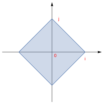
In linear algebra, functional analysis, and related areas of mathematics, a norm is a function that assigns a strictly positive length or size to each vector in a vector space—save for the zero vector, which is assigned a length of zero.
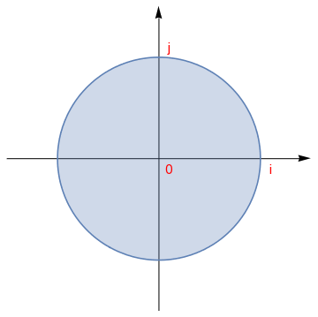
On an n-dimensional complex space \( \mathbb{C}^n ,\) the most common norm is
A unit vector u is a vector whose length equals one: \( {\bf u} \cdot {\bf u} =1 . \) We say that two vectors
x and y are perpendicular if their dot product is zero.
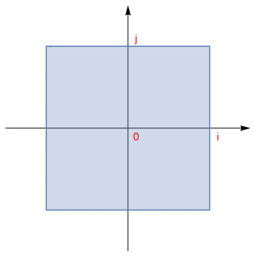
There are known many other norms.
The inequality for sums was published by the French mathematician and physicist Augustin-Louis Cauchy (1789--1857) in 1821, while the corresponding
inequality for integrals was first proved by the Russian mathematician Viktor Yakovlevich Bunyakovsky (1804--1889) in 1859. The modern proof
(which is actually a repetition of the Bunyakovsky's one) of the integral inequality was given by the German mathematician Hermann Amandus Schwarz (1843--1921) in 1888.
With Euclidean norm, we can define the dot product as