The Gaussian
elimination method is one of the most important and ubiquitous
algorithms that can help
deduce important information about the given matrix�s roots/nature as well
determine the solvability of linear system when it is applied to the augmented
matrix. As such, it is one of the most useful numerical algorithms and
plays a fundamental role in scientific computation. This method has
been historically around and used by Chinese mathematicians since, 179 CE.
Many people have contributed to Gaussian elimination, including Isaac Newton.
However, it was named by the American mathematician George Forsythe (1917--1972) in honor of the German mathematician
and physicist Carl Friedrich Gauss (1777--1855). The full history of Gaussian algorithm can be found within the Joseph F. Grcar
article.
For our exposition, we need a shorthand way of writing systems of equations.
For a linear system of equation Ax = b, where A is an
m×n matrix and b is a known n column vector,
we assign the m×(n+1)augmented matrix, denoted [A|b] or (A|b), which
is A with column b tagged on.
Sometimes a vertical line is used to separate the coefficient entries from the
constants can be dropped and then augmented matrix is written as
[Ab] .
The augmented matrix provides a precise and concise information about a linear
system of equations
A system of linear equations above, written in compact vector form
Ax = b, is said to be consistent if it has at least one solution and inconsistent if there is no solution.
To understand the idea of Gaussian elimination algorithm, we shall consider a series
of examples, starting with a two dimensional case.
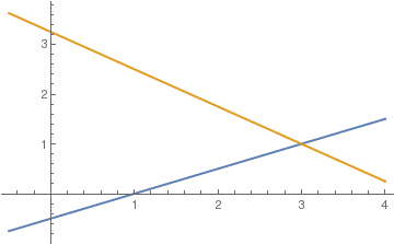
Example: Consider the system of algebraic equations
\begin{align*}
x -2\, y &= 1 , \\
3\,x + 4\,y &= 13 .
\end{align*}
If we multiply the first equation by -3 and add to the last one (which does
not change the solution), we get
\[
{\bf Before: } \quad
\begin{split}
x -2\, y &= 1 , \\
3\,x + 4\,y &= 13 ;
\end{split} \qquad {\bf After: } \quad
\begin{split}
x -2\, y &= 1 , \\
\qquad\qquad 10\,y &= 10 ;
\end{split} \qquad
\begin{split}
\mbox{(multiply by 3 and subtract)} \\
(x\mbox{ has been eliminated)}
\end{split}
\]
The first stage we accomplished is called forward elimination
because it deleted one variable from consideration. Forward elimination
produces an upper triangular system, which can be seen with
matrix notation (which is called the augmented matrix).
The last equation 10y = 10 reveals y = 1, and we go up the
triangle to x = 3. This quick process is called
back substitution. It is used for upper triangular systems of any size,
after forward elimination is complete. We plot our equations with
Mathematica.
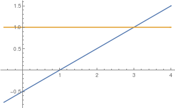
Two lines after eliminating variable y.
Which variable should you eliminate, x or y? For a computer, it does not matter, but for humans it does because it is simpler. So mostly for educational purposes, we will follow tradition and we will eliminate variables from left to right in order to reduce the matrices into upper triangular form. However, remember that when you write code for practical calculations, it does not matter which variable you eliminate and in what order---the computer does not care!
When we used matrix form corresponding to the given system of equations, we
marked with the color red for special positions in the corresponding augmented matrix
because they are important to understand. These positions are usually referred to as pivots.
■
Example: Now we consider slightly different
system of algebraic equations
\begin{align*}
x -2\, y &= 1 , \\
3\,x - 6\,y &= 13 .
\end{align*}
Eliminating variable x by subtracting 3 times first equation from the
second one, we obtain
\begin{align*}
x -2\, y &= 1 , \\
0\,x - 0\,y &= \color{red}{10} .
\end{align*}
There is no solution. Remember that zero is never allowed as a pivot, hence
we get an equation with a pivot at the last column.
The last line in the matrix shows that every x and y satisfy the
equation 0·x + 0·y = 0. There is really only one
equation x - 2y = 1. One of the variables is free when another
one is expressed through the free one:
\[
x = 1 + 2\,y \qquad \mbox{or} \qquad y = \left( x-1 \right) /2 ,
\]
when y or x is freely chosen, respectively. There is no need to
plot one straight line that includes both equations because every its point
satisfies both equations. We have a whole line of solutions.
■
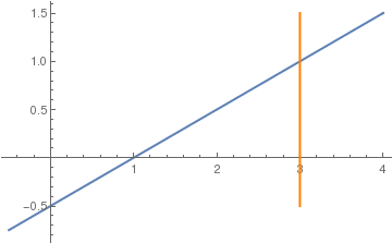
Example: Consider the system of algebraic equations
For this system, we cannot choose the first coefficient as a pivot because by
definition the pivot cannot be zero. So exchange two equations to obtain an
equivalent augmented matrix:
Two lines intersect at one point (3,1).
The new system is already triangular, so one of the lines is parallel to an
axis.
■
To understand Gaussian elimination, you have to go beyond 2�2 systems of
equations. Therefore, we present examples of 3�3 systems of equations that will
be enough to see the pattern. The other example, with rectangular matrices, is
following.
Example: Consider the system of algebraic equations
This matrix contains all of the information in the system of equations without
the unknown variables x, y, and z to carry around. Now
we perform the process of elimination. The notation to the right of each
matrix describes the row operations that were performed to get the matrix on
that line. For example 2R1+R2 ↦ R2 means
"replace row 2 with the sum of 2 times row 1 and row 2."
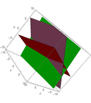
Planes in the echelon form.
We can now easily solve for x, y, and z by
back-substitution to obtain x = 1, y = -2, and
z = -1.
For a system of equations with a 3x3 matrix of coefficients, the goal of the process of Gaussian Elimination is to create (at least) a triangle of zeroes in the lower left hand corner of the matrix below the diagonal. Note that you may switch the order of the rows at any time in trying to get to this form.
a1 = ContourPlot3D[x - 3 y + z == 6,
{x, -10, 10}, {y, -10, 10}, {z, -10, 10},
AxesLabel -> {x, y, z}, Mesh -> None, ContourStyle -> Directive[Red]];
f2[x_, y_] := (-2* x + y-1)/5;
a2 = ParametricPlot3D[{x, y, f2[x, y]},
{x, -10, 10}, {y, -10, 10},
AxesLabel -> {x, y, z}, Mesh -> None, PlotStyle -> Directive[Green]];
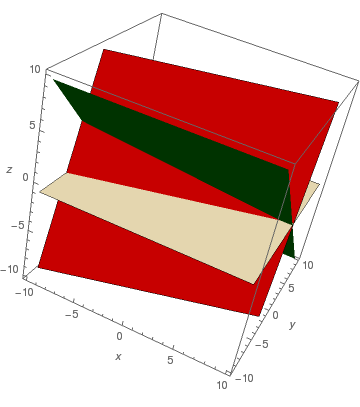
No solution.
We keep x in the first equation and eliminate it from the other
equations. To do so, add -1 times equation 1 to equation 2. After some
practice, this type of calculation is usually performed mentally. However,
it is convenient to use software:
Notice the last equation reads: 0=5. This is not possible. So the system has
no solutions; it is not possible to find values x, y, and
z that satisfy all three equations simultaneously.
■
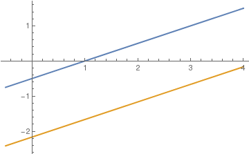
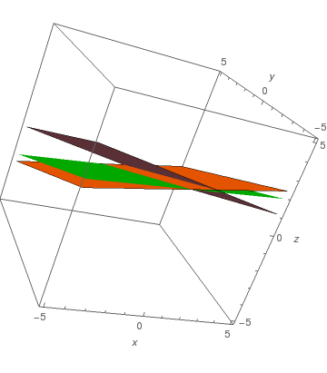
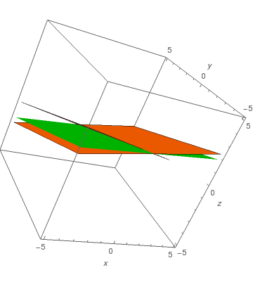
Example: Consider the system of algebraic equations
Notice the last equation: 0=0 (this resulted from equation 3 being a linear
combination of the other two equations). This is always true. And, we can
solve the first two equations to get x and y as functions of
z alone. Solving these equations, we get
To eliminate x1 from the last three equations, we multiply
the first equation by -1, -2, and 3, respectively. By adding the results to
the corresponding rows, it will introduce zeroes into positions below the pivot
(which we mark with red) in the first column:
Finally, multiplying the third row by 8 and adding to the last row, we obtain,
what is usually called the row echelon form for the given augmented matrix:
The Gaussian elimination method is basically a series of operations carried
out on a given matrix, in order to mathematically simplify it to its echelon
form. When it is applied to solve a linear system Ax=b, it
consists of two steps: forward elimination (also frequently called
Gaussian
elimination procedure) to reduce the matrix to upper triangular form,
and back substitution. Therefore, solving a linear system of algebraic equations using this elimination procedure can also be called forward elimination and back substitution and abbreviated as FEBS.
A rectangular matrix is said to be in echelon form or row echelon form
if it has the following three properties:
All nonzero rows are above any rows of all zeroes.
Each leading entry, called the pivot, of a row is in a column to
the right of the leading entry of the row above it.
All entries in a column below a leading entry are zeroes.
An echelon matrix is one that is in echelon form.
A matrix is said to be in its row echelon form when it meets the following two
conditions:
Any present zero rows are placed all the way at the bottom of the
matrix.
The very first value of the matrix (termed as the leading entry or
pivot) is a non-zero term (some texts prefer it be �1�, but it is not
necessarily).
Example: The following matrices are in the echelon
form:
where ♦ denotes the pivot's position (the entry cannot be zero),
* denotes arbitrary element that could be zero or not, and ⊚ denotes
lonely nonzero entry that looks as a pivot but it indicates that the
corresponding system has no solution. From theoretical point of view, a pivot
could be in the last column, but when dealing with augmented matrices
corresponding to the linear system of equations, we avoid this. For consistent
systems, pivots cannot be in lonely position at the end of a row; otherwise,
the system has no solution.
■
A pivot position in a matrix A is a location in A that
corresponds to a leading term in the row echelon form of A. A
pivot column is a column of A that contains a pivot position.
Any nonzero matrix may be row reduced (that is, transformed by
elementary row operations) into more than one matrix in echelon form, using
different sequences of row operations. However, the leading entries are always
in the same positions in any echelon form obtained from a given matrix.
Theorem: A linear system has a solution
if and only if the rightmost column of the associated augmented matrix is
not a pivot column---that is, if and only if its echelon form does not
contain a row of the form
[ 0 0 ... 0 ⊚ ] with ⊚ nonzero.
If a linear system is consistent, then the solution set contains either a
unique solution (with no free variables) or infinitely many solutions, when
there is at least one free variable.
Row echelon form states that the Gaussian elimination method has been
specifically applied to the rows of the matrix. It uses only those operations
that preserve the solution set of the system, known as elementary row
operations:
Addition of a multiple of one equation to another. Symbolically: (equation j) \( \mapsto \) (equation j) + k (equation i).
Multiplication of an equation by a nonzero constant k. Symbolically: (equation j) \( \mapsto \) k (equation j).
Interchange of two equations> Symbolically: (equation j) \( \Longleftrightarrow \) (equation i).
Maxime B�cher
Row echelon and Reduced row echelon forms are the resulting
matrices of the Gaussian elimination method. By applying Gaussian elimination
to any matrix, one can easily deduce the following information about the
given matrix:
the rank of the matrix;
the determinant of the matrix;
the inverse (invertible square matrices only);
the kernel vector (also known as �null vector�).
The main purpose of writing a matrix in its row echelon form and/or reduced
row echelon, is to make it easier to examine the matrix and to carry out
further calculations, especially when solving a system of algebraic equations.
When forward elimination procedure is applied to a system of algebraic
equations Ax=b, the first step is create an
augmented matrix,
which is obtained by appending the columns vector b from right to the
matrix of the system:
\( {\bf B} = \left[ {\bf A} \, \vert \, {\bf b} \right] . \) The next step is to use elementary row operations to reduce the
augmented matrix B to the new augmented matrix
\( {\bf C} = \left[ {\bf U} \, \vert \, {\bf c} \right] , \) where U is upper triangular matrix. This means that the new
system Ux=c is easy to solve.
The actual use of the term augmented matrix was evolved by the American
mathematician
Maxime B�cher
(1867--1918) in his book
Introduction to Higher Algebra, published in 1907. B�cher was an
outstanding expositor of mathematics whose elementary textbooks were greatly
appreciated by students. His achievements were documented by
William F. Osgood (1919).
Variables in a linear system of equations that corresponds to pivot positions
in the augmented matrix for the given system are called the
leading variables. the remaining variables are called
free variables.
Example: We consider the following
augmented matrix:
This matrix corresponds to four equations in six unknown variables. Since
pivots are located in columns 1, 3, and 6, the leading variables for this
system of equations are x1, x3, and
x6. The other three variables x2,
x4, and x5 are free variables.
■
Theorem:
If a homogeneous linear system has n unknowns, and if the row echelon
form of its augmented matrix has r nonzero rows, then the system has
n-r free variables.
Row operations can be applied to any matrix, not merely to one that arises as
the augmented matrix of a linear system. Two matrices are called
row equivalent if there is a sequence of elementary row operations that transforms one matrix into the other. It is important to note that row operations are reversible. if two rows are interchanged, they can be returned to their original positions by another interchange. If a row scaled is scaled by a nonzero constant k, then multiplying the new row by 1/k produces the original row. Finally, consider a replacement operation involving two rows---say 1 and 3---and suppose that k times row 1 is added to row 3 to obtain a new row 3. To come back, just add -k times row 1 to new row 3 and you will get the original row 3.
Theorem: Let
\( {\bf B} = \left[ {\bf A} \, \vert \, {\bf b} \right] \)
be the augmented matrix corresponding to the linear equation
Ax=b, and suppose B is row equivalent (using a sequence
of elementary row operations) to the
new augmented matrix \( {\bf C} = \left[ {\bf U} \, \vert
\, {\bf c} \right] , \) which corresponds to the linear system
Ux=c. Then the two linear systems have precisely the same
solution set.
Naive Gaussian elimination algorithm for Ax=b with a square
matrix A (pseudocode)
for i=1 to n-1
	for j=i+1 to n
		m=a(j,i)/a(i,i)
		for k=i+1 to n
			a(j,k) = a(j,k) -m&a(i,k)
		endfor
		b(j) = b(j) - m*b(i)
	endfor
endfor
The outmost loop (the i loop) ranges over the columns of the matrix;
the last column is skipped because we do not need to perform any eliminations
there because there are no elements below the diagonal (if we were doing
elimination on a nonsquare matrix with more rows than columns, we would have
to include the last column in this loop).
The middle loop (the j loop) ranges down the i-th column, below
the diagonal (hence j ranges only from i+1 to n---the
dimension of the matrix A). We first compute the
multiplierm, for each row. This is the constant by which we
multiply the i-th row in order to eliminate the aji
element. Note that we overwrite the previous values with the new ones,
and we do not actually carry out computation that makes aji
zero. Also this loop is where the right-side vector is modified to reflect the
elimination step.
The innermost loop (the k loop) ranges across the j-th row,
starting after the i-th column, modifying each element appropriately to
reflect the elimination of aji.
Finally, we must be aware that the algorithm does not actually create the
zeroes in the lower triangular half of B; this would be wasteful of
computer time since we don't need t have these zeroes in place for the
algorithm to work. The algorithm works because we utilize only the upper
triangular part of the matrix from this point forward, so the lower triangular
elements need never be referenced.
Backward solution algorithm for A (pseudocode)
x(n) = b(n)/a*n,n)
for i=n-1 to 1
	sum = 0
	for j=i+1 to n
		sum = sum + a(i,j)*x(j)
	endfor
	x(i) = (b(i) - sum)/a(i,i)
endfor
This algorithm simply matches backward up the diagonal, computing each
xi in turn. Finally, we are computing
which is what is necessary to solve a triangular system. The j loop is
simply accumulating the summation term in this formula. The algorithm stops if
one of the diagonal terms is zero because we cannot divide by it. This case
requires a special attention that yields interchange of row.
The idea of Gaussian elimination is to replace the above system by another
system with the same solutions, it is just easier to solve. First, we build
the augmented matrix corresponding to the given system of equations:
Therefore, we obtain an equivalent augmented matrix in row echelon form. Since
it contains one row of all zeroes, the given system has infinite many solutions
that we obtain by solving the second equation:
\[
6\,y + 4\,z = -1 \qquad \Longrightarrow \qquad z = - \frac{3}{2}\, y -
\frac{1}{4} .
\]
Using this expression, we get from the first equation
We apply the same procedure as in the previous example: forward elimination.
The procedure to be used expresses some of unknowns in terms of others by
eliminating certain unknowns from all the equations except one. To begin, we
eliminate x from every equation except the first one by adding -2/3
times the first equation to the second and 1/3 times the first equation to the
third. The result is the following new system:
Since the pivot is situated in the last column of the augmented matrix, the
given system of equations has no solution because it is impossible to satisfy
the equation 0 = 2.
Example:
When using the Gaussian elimination technique, you can at any time exchange
rows, meaning that you can switch any two rows an unlimited number of times.
This is very helpful if your matrix contains a 0 in the (1,1) position.