In this section, we discuss some algorithms to solve numerically boundary value porblems for Laplace's equation (∇2u = 0), Poisson's equation (∇2u = g(x,y)), and Helmholtz's equation (∇2u + k(x,y) u = g(x,y)). We start with the Dirichlet problem in a rectangle \( R = [0,a] \times [0,b] . \)
Actually, matlab has a special Partial Differential Equation Toolbox to solve some partial differential equations using finite element analysis including the heat transfer equations and Laplace's equations under various boundary conditions. The explanation how to use it is provided on Mathworks site. We demonstrait its applications in some examples below.
The Laplacian operator must be expressed in a discrete form suitable for numerical computations. The formula for approximating \( f'' (x) \) is obtained from
\[
f'' (x) = \frac{f(x+h) -2\,f(x) + f(x-h)}{h^2} +O(h^2 ) .
\]
When this formula is applied to the Laplace equation involving approximation of partial derivatives
uxx and
uyy and the results are added, we obtain
\[
\Delta u = \frac{1}{h^2} \left[ u(x+h,y) + u(x-h,y) + u(x,y+h) + u(x,y-h) -4\,u(x,y) \right] +O(h^2 ) .
\]
Suppose that we seek a solution of the Laplace equation in the rectangular domain [0,a]×[0,b]. Assume that the rectangle is divided into (
n-1)×(
m-1) squares with side
h so that
a =
nh and
b =
mh because we assume also that
b/a = m/n.
l0 = Graphics[{Thick,Line[{{0,0},{8,0}}]}];
l1 = Graphics[{Thick,Line[{{0,1},{8,1}}]}];
l2 = Graphics[{Thick,Line[{{0,2},{8,2}}]}];
l3 = Graphics[{Thick,Line[{{0,3},{8,3}}]}];
l4 = Graphics[{Thick,Line[{{0,4},{8,4}}]}];
l5 = Graphics[{Thick,Line[{{0,5},{8,5}}]}];
la0 = Graphics[{Thick,Line[{{0,0},{0,5}}]}];
la1 = Graphics[{Thick,Line[{{1,0},{1,5}}]}];
la2 = Graphics[{Thick,Line[{{2,0},{2,5}}]}];
la3 = Graphics[{Thick,Line[{{3,0},{3,5}}]}];
la4 = Graphics[{Thick,Line[{{4,0},{4,5}}]}];
la5 = Graphics[{Thick,Line[{{5,0},{5,5}}]}];
la6 = Graphics[{Thick,Line[{{6,0},{6,5}}]}];
la7 = Graphics[{Thick,Line[{{7,0},{7,5}}]}];
la8 = Graphics[{Thick,Line[{{8,0},{8,5}}]}];
d0 = Graphics[{Orange, Disk[{4, 3}, 0.15]}];
d1 = Graphics[{Orange, Disk[{4, 4}, 0.15]}];
d2 = Graphics[{Orange, Disk[{4, 2}, 0.15]}];
d3 = Graphics[{Orange, Disk[{3, 3}, 0.15]}];
d4 = Graphics[{Orange, Disk[{5, 3}, 0.15]}];
r1 = Graphics[
Text[Style["\!\(\*SubscriptBox[\(x\), \(i\)]\)",
Medium], {4, -0.3}]];
r2 = Graphics[
Text[Style["\!\(\*SubscriptBox[\(x\), \(i-1\)]\)",
Medium], {3, -0.3}]];
r3 = Graphics[
Text[Style["\!\(\*SubscriptBox[\(x\), \(i+1\)]\)",
Medium], {5, -0.3}]];
r4 = Graphics[
Text[Style["\!\(\*SubscriptBox[\(x\), \(n-1\)]\)",
Medium], {7, -0.3}]];
r5 = Graphics[
Text[Style["\!\(\*SubscriptBox[\(x\), \(n\)]\)",
Medium], {8, -0.3}]];
r6 = Graphics[
Text[Style["\!\(\*SubscriptBox[\(x\), \(2\)]\)",
Medium], {1, -0.3}]];
r7 = Graphics[
Text[Style["\!\(\*SubscriptBox[\(x\), \(1\)]\)",
Medium], {0, -0.3}]];
t0 = Graphics[
Text[Style["\!\(\*SubscriptBox[\(y\), \(1\)]\)",
Medium], {-0.3, 0}]];
t1 = Graphics[
Text[Style["\!\(\*SubscriptBox[\(y\), \(j-1\)]\)",
Medium], {-0.4, 2}]];
t2 = Graphics[
Text[Style["\!\(\*SubscriptBox[\(y\), \(j\)]\)",
Medium], {-0.3, 3}]];
t3 = Graphics[
Text[Style["\!\(\*SubscriptBox[\(y\), \(j+1\)]\)",
Medium], {-0.4, 4}]];
t4 = Graphics[
Text[Style["\!\(\*SubscriptBox[\(y\), \(m\)]\)",
Medium], {-0.3, 5}]];
Show[l0,l1,l2,l3,l4,l5,la0,la1,la2,la3,la4,la5,la6,la7,la8,d0, d1, d2, d3, d4, r1,r2,r3,r4,r5,r6,r7, t0,t1,t2,t3,t4]
The grid used with Laplace's difference equation
To solve Laplace's equation, we impose the approximation
\[
\frac{1}{h^2} \left[ u(x+h,y) + u(x-h,y) + u(x,y+h) + u(x,y-h) -4\,u(x,y) \right] =0,
\]
which has order of accuracy O(
h2) at all interior grid points
\( (x,y) = (x_i , y_j ) \) for
i = 2, 3, …,
n-1 and
j = 2, 3, …,
m-1. The grid points are uniformly spaced:
\( x_{i+1} = x_i + h, \ x_{i-1} = x_i -h, \ y_{j+1} = y_j +h , \ y_{j-1} = y_j -h . \) Using notation
ui,j for
\( u (x_i , y_j ) , \) the discrete Laplace equation can be written as
\[
\Delta u_{i,j} \approx \frac{u_{i+1,j} + u_{i-1,j} + u_{i,j+1} + u_{i,j-1} - 4\,u_{i,j}}{h^2} =0 ,
\]
which is known as the
five-point difference formula for Laplace's equation. This formula is usually called the
five-point stencil of a point in the grid is a
stencil made up of the point itself together with its four "neighbors". It is used to write
finite difference approximations to
derivatives at grid points. This formula relates the function value
\( u_{i+1,j} \equiv u(x_{i+1}, y_j ) \) to its four neighboring values
ui+1,j,
ui-1,j,
ui,j+1, and
ui,j-1, as shown in stencil below. The multiple
h2 can be eliminated and we obtain the
Laplacian computational formula:
\[
u_{i+1,j} + u_{i-1,j} + u_{i,j+1} + u_{i,j-1} - 4\,u_{i,j} =0 .
\]
l1 = Graphics[{Thick,Line[{{-2,0},{2,0}}]}];
l2 = Graphics[{Thick,Line[{{0,-2},{0,2}}]}];
d0 = Graphics[{Red, Disk[{0, 0}, 0.1]}];
d1 = Graphics[{Blue, Disk[{0, 2}, 0.1]}];
d2 = Graphics[{Blue, Disk[{0, -2}, 0.1]}];
d3 = Graphics[{Blue, Disk[{2, 0}, 0.1]}];
d4 = Graphics[{Blue, Disk[{-2, 0}, 0.1]}];
t0 = Graphics[
Text[Style["\!\(\*SubscriptBox[\(-4 u\), \(i,j\)]\)",
Medium], {0.4, -0.2}]];
t1 = Graphics[
Text[Style["\!\(\*SubscriptBox[\(u\), \(i-1,j\)]\)",
Medium], {-2.2, -0.2}]];
t2 = Graphics[
Text[Style["\!\(\*SubscriptBox[\(u\), \(i+1,j\)]\)",
Medium], {2.2, -0.2}]];
t3 = Graphics[
Text[Style["\!\(\*SubscriptBox[\(u\), \(i,j+1\)]\)",
Medium], {0.2, 2.2}]];
t4 = Graphics[
Text[Style["\!\(\*SubscriptBox[\(u\), \(i,j-1\)]\)",
Medium], {-0.2, -2.2}]];
Show[l1,l2,d0,d1,d2,d3,d4, t0,t1,t2,t3,t4]
The Laplace stencil
Assume that the values u(x,y) are known at the following boundary grid points:
\begin{align*}
u(x_1,y_j ) &= u_{1,j} \qquad&\mbox{for } 2 \le j \le m-1 \qquad &(\mbox{on the left}), \\
u(x_i, y_1 ) &= u_{i,1} \qquad&\mbox{for } 2 \le i \le n-1 \qquad &(\mbox{on the bottom}), \\
u(x_n,y_j ) &= u_{1,j} \qquad&\mbox{for } 2 \le j \le m-1 \qquad &(\mbox{on the right}), \\
u(x_i, y_m ) &= u_{i,1} \qquad&\mbox{for } 2 \le i \le n-1 \qquad &(\mbox{on the top}) .
\end{align*}
Then applying the Laplace computational formula at each of the interior points of
R will creat a linear system of (
n-2) equations in (
n-2) unknowns, which is solved to obtain approximations to
u(x,y) at the interior points of
R.
Program (Dirichlet method for Laplace's equation): to approximate the solution of \( u_{xx} + u_{yy} =0 \) over \( R = \{\,(x,y) \,:\, 0 \le x \le a , \ 0 \le y \le b \) with \( u(x,0) = f_0 (x), \ u(x,b) = f_b (x) , \) for 0 ≤ x ≤ a;, and \( u(0,y) = g_0 (y), \ u(a,y) = g_a (y) , \) for 0 ≤ y ≤ b. It is assumed that Δx = Δy = h and that integers n and m exist so that a=nh and b=mh.
function U=dirichlet(f0,fb,g0,ga,a,b,h,tol,max1)
% Input  -- f0,fb,g0,ga are boundary functions input as a strings
%        -- a and b right end points of [0,a] and [0,b]
%        -- h step size
%        -- tol is the tolerance
%        -- max1
% Output -- U solution matrix;
% Initialize parameters and U
n=fix(a/h)+1;
m=fix(b/h)+1;
ave=(a*(feval(f0,0)+feval(fb,0))+b*(feval(g0,0)+feval(ga,0)))/(2*a+2*b);
U=ave*ones(n,m);
% Boundary conditions
U(1,1:m)=feval(g0,0:h:(m-1)*h))';
U(n,1:m)=feval(ga,0:h:(m-1)*h))';
U(1:n,1)=feval(fa,0:h:(n-1)*h))';
U(1:n,m)=feval(fb,0:h:(n-1)*h))';
U(1,1)=(U(1,2)+U(2,1))/2;
U(1,m)=(U(i,m-1)+U(2,m))/2;
U(n,1)=(U(n-1,1)+U(n,2))/2;
U(n,m)=(U(n-1,m)+U(n,m-1))/2;
% SQR parameter
w=4/(2+sqrt(4-(cos(pi/(n-1))+cos(pi/(m-1)))^2));
% Refine approximations and sweep operator throughout the grid
err=1;
cnt=0;
while((err>tol)&(cnt<=max1))
    err=0;
    for j=2:m-1
        for i=2:n-1
            relx=w*(U(i,j+1)+U(i,j-1)+U(i+1,j)+U(i-1,j)-4*U(i,j))/4;
            U(i,j)=U(i,j)+relx;
            if (err<=abs(relx))
            err=abs(relx);
            end
         end
     end
cnt=cnt+1;
end
U=flipud(U');
l0 = Graphics[{Thick,Line[{{0,0},{10,0}}]}];
l1 = Graphics[{Thick,Line[{{0,0},{0,8}}]}];
l2 = Graphics[{Thick,Line[{{0,8},{10,8}}]}];
l3 = Graphics[{Thick,Line[{{10,0},{10,8}}]}];
d0 = Graphics[{Blue, Disk[{0, 2}, 0.15]}];
d1 = Graphics[{Blue, Disk[{0, 4}, 0.15]}];
d2 = Graphics[{Blue, Disk[{0, 6}, 0.15]}];
d3 = Graphics[{Blue, Disk[{2, 0}, 0.15]}];
d4 = Graphics[{Blue, Disk[{2, 2}, 0.15]}];
d5 = Graphics[{Blue, Disk[{2, 4}, 0.15]}];
d6 = Graphics[{Blue, Disk[{2, 6}, 0.15]}];
d7 = Graphics[{Blue, Disk[{2, 8}, 0.15]}];
d8 = Graphics[{Blue, Disk[{4, 0}, 0.15]}];
d9 = Graphics[{Blue, Disk[{4, 2}, 0.15]}];
d10 = Graphics[{Blue, Disk[{4, 4}, 0.15]}];
d11 = Graphics[{Blue, Disk[{4, 6}, 0.15]}];
d12 = Graphics[{Blue, Disk[{4, 8}, 0.15]}];
d13 = Graphics[{Blue, Disk[{6, 0}, 0.15]}];
d14 = Graphics[{Blue, Disk[{6, 2}, 0.15]}];
d15 = Graphics[{Blue, Disk[{6, 4}, 0.15]}];
d16 = Graphics[{Blue, Disk[{6, 6}, 0.15]}];
d17 = Graphics[{Blue, Disk[{6, 8}, 0.15]}];
d18 = Graphics[{Blue, Disk[{8, 0}, 0.15]}];
d19 = Graphics[{Blue, Disk[{8, 2}, 0.15]}];
d20 = Graphics[{Blue, Disk[{8, 4}, 0.15]}];
d21 = Graphics[{Blue, Disk[{8, 6}, 0.15]}];
d22 = Graphics[{Blue, Disk[{8, 8}, 0.15]}];
d23 = Graphics[{Blue, Disk[{10, 2}, 0.15]}];
d24 = Graphics[{Blue, Disk[{10, 4}, 0.15]}];
d25 = Graphics[{Blue, Disk[{10, 6}, 0.15]}];
r1 = Graphics[
Text[Style["\!\(\*SubscriptBox[\(u\), \(2,1\)]\)",
Medium], {2, -0.5}]];
r2 = Graphics[
Text[Style["\!\(\*SubscriptBox[\(u\), \(3,1\)]\)",
Medium], {4, -0.5}]];
r3 = Graphics[
Text[Style["\!\(\*SubscriptBox[\(u\), \(4,1\)]\)",
Medium], {6, -0.5}]];
r4 = Graphics[
Text[Style["\!\(\*SubscriptBox[\(u\), \(5,1\)]\)",
Medium], {8, -0.5}]];
r5 = Graphics[
Text[Style["\!\(\*SubscriptBox[\(u\), \(1,2\)]\)",
Medium], {-0.8, 2.0}]];
r6 = Graphics[
Text[Style["\!\(\*SubscriptBox[\(u\), \(1,3\)]\)",
Medium], {-0.8, 4}]];
r7 = Graphics[
Text[Style["\!\(\*SubscriptBox[\(u\), \(1,4\)]\)",
Medium], {-0.8, 6}]];
r8 = Graphics[
Text[Style["\!\(\*SubscriptBox[\(u\), \(6,2\)]\)",
Medium], {10.8, 2}]];
r9 = Graphics[
Text[Style["\!\(\*SubscriptBox[\(u\), \(6,3\)]\)",
Medium], {10.8, 4}]];
r10 = Graphics[
Text[Style["\!\(\*SubscriptBox[\(u\), \(6,4\)]\)",
Medium], {10.8, 6}]];
r11 = Graphics[
Text[Style["\!\(\*SubscriptBox[\(u\), \(1,4\)]\)",
Medium], {2, 8.6}]];
r12 = Graphics[
Text[Style["\!\(\*SubscriptBox[\(u\), \(6,2\)]\)",
Medium], {4, 8.6}]];
r13 = Graphics[
Text[Style["\!\(\*SubscriptBox[\(u\), \(6,2\)]\)",
Medium], {6, 8.6}]];
r14 = Graphics[
Text[Style["\!\(\*SubscriptBox[\(u\), \(6,2\)]\)",
Medium], {8, 8.6}]];
t0 = Graphics[
Text[Style["\!\(\*SubscriptBox[\(p\), \(1\)]\)",
Medium], {2, 1.5}]];
t1 = Graphics[
Text[Style["\!\(\*SubscriptBox[\(p\), \(2\)]\)",
Medium], {4, 1.5}]];
t2 = Graphics[
Text[Style["\!\(\*SubscriptBox[\(p\), \(3\)]\)",
Medium], {6, 1.5}]];
t3 = Graphics[
Text[Style["\!\(\*SubscriptBox[\(p\), \(4\)]\)",
Medium], {8, 1.5}]];
t4 = Graphics[
Text[Style["\!\(\*SubscriptBox[\(p\), \(5\)]\)",
Medium], {2, 3.5}]];
t5 = Graphics[
Text[Style["\!\(\*SubscriptBox[\(p\), \(6\)]\)",
Medium], {4, 3.5}]];
t6 = Graphics[
Text[Style["\!\(\*SubscriptBox[\(p\), \(7\)]\)",
Medium], {6, 3.5}]];
t7 = Graphics[
Text[Style["\!\(\*SubscriptBox[\(p\), \(8\)]\)",
Medium], {8, 3.5}]];
t8 = Graphics[
Text[Style["\!\(\*SubscriptBox[\(p\), \(9\)]\)",
Medium], {2, 5.5}]];
t9 = Graphics[
Text[Style["\!\(\*SubscriptBox[\(p\), \(10\)]\)",
Medium], {4, 5.5}]];
t10 = Graphics[
Text[Style["\!\(\*SubscriptBox[\(p\), \(11\)]\)",
Medium], {6, 5.5}]];
t11 = Graphics[
Text[Style["\!\(\*SubscriptBox[\(p\), \(12\)]\)",
Medium], {8, 5.5}]];
Show[l0,l1,l2,l3,d0,d1, d2, d3, d4,d5,d6,d7,d8,d9,d10,d11,d12,d13,d14,d15,d16,d17,d18,d19,d20,d21,d22,d23,d24,d25, r1,r2,r3,r4,r5,r6,r7, t0,t1,t2,t3,t4,t5,t6,t7,t8,t9,t10,t11]
A 5×6 gtid for boundary values only
For example, suppose that the region is a rectangle with n=6 and m=5, and that the unknown values of u(xi,yj) at the twelve interior grid points are labeled p1, p2, ... ,p12 and positioned in the grid as shown in the figure above. The Laplacian computational formula is applied at each of the interior grid points, and the result is the system A p = b of twelve linear equations:
\begin{align*}
-4\,p_1 + p_2 + p_4 &= -u_{2,1} - u_{1,2} \\
p_1 -4\,p_2 + p_3 + p_5 &= -u_{3,1} , \\
\end{align*}
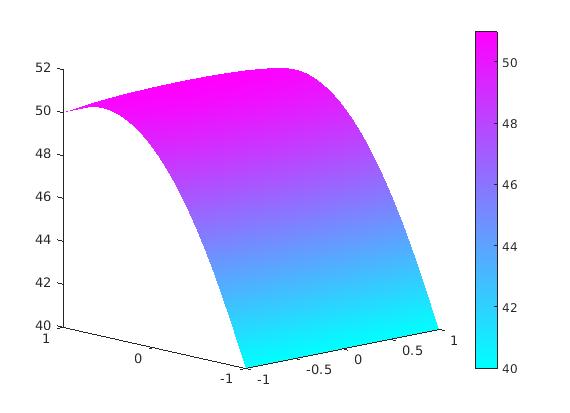
Example 1:
Consider the Laplace equation in a square subject to the mixd boundary conditions
\begin{align*}
&\mbox{Laplace equation:} \qquad &u_{xx} + u_{yy} &= 0 \qquad\mbox{for } -1 < x < 1 \mbox{ and } -1 < y < 1, \\
&\mbox{Dirichlet boundary conditions on }x: \qquad &u(-1,y) &= 50 , \quad \mbox{and} \quad u(1,y) = 40, \\
&\mbox{Neumann boundary condition on }y: \qquad &u_y(x,0) &= 1 , \quad \mbox{and} \quad u_y (x,1) = -1, \\
&\mbox{Corner regularity condition:} && \mbox{function } u(x,y) \quad \mbox{is bounded at every corner point}.
\end{align*}
To solve this problem numerically, we use
matlab special
tool box for solving PDEs with constant boundaey conditions.
|
|
Using matlab toolbox for solving the given boundary value problem with constant mixed boundary conditions:
model = createpde;

geometryFromEdges(model,@squareg); % takes the geometry of a square
pdegplot(model,'EdgeLabels','on')
xlim([-1.1,1.1]) % limits to x values beyond where our object lies
axis equal

applyBoundaryCondition(model,'dirichlet','edge',3,'u',40); % edge 3 has a dirichlet value of 40
applyBoundaryCondition(model,'dirichlet','edge',1, 'u', 50);% edge 1 has a dirichlet value of 50
applyBoundaryCondition(model,'neumann','edge',[2,4], 'g', -1); % neumann conditions on edge 2 and 4 value of -1

specifyCoefficients(model,'m',0,'d',0,'c',1,'a',0,'f',10);% see attached document, these are the same conditions used in the mathWorks example
generateMesh(model,'HMax', 0.1); % affects the smoothness of the plot
results = solvepde(model);
u = results.NodalSolution;
pdeplot(model,'XYData', u, 'ZData', u)
|
|
Solution of Laplace's equation.
|
|
matlab code.
|
■
For non-constant boundary conditions, matlab has a special toolbox.
To solve problems using PDEModel 0bjects, please follow
web page that gives the general explanation of PDESolver.
The cor4esponing mesh and geometry explanation is given on the
web.