Suppose that A is a diagonalizable \( n \times n \) matrix; this means that all its eigenvalues are not defective and there exists a basis of n linearly independent eigenvectors. Now assume that its minimal polynomial (the polynomial of least possible degree that anihilates the matrix) is a product of simple terms:
Let \( f(\lambda ) \) be a function defined on the spectrum of the matrix A. The last condition means that every eigenvalue λi is in the domain of f, and that every eigenvalue λi with multiplicity mi > 1 is in the interior of the domain, with f being (mi — 1) times differentiable at λi. We build a function \( f\left( {\bf A} \right) \) of diagonalizable square matrix A according to James Sylvester, who was an English lawyer and music tutor before his appointment as a professor of mathematics in 1885. To define a function of a square matrix, we need to construct k Sylvester auxiliary matrices for each distinct eigenvalue \( \lambda_i , \quad i= 1,2,\ldots k: \)
Each Sylvester's matrix is a projection matrix on eigenspace of the corresponding eigenvalue.
Example 1.7.1: Consider the \( 3 \times 3 \) matrix \( {\bf A} = \begin{bmatrix} 1&4&16 \\ 18&20&4 \\ -12&-14&-7 \end{bmatrix} \) that has three distinct eigenvalues Then we define the resolvent, \( {\bf R}_{\lambda} ({\bf A} ) = (\lambda {\bf I} - {\bf A})^{-1} : \)
% 3x3 matrix with 2 distinct real eigenvalues
syms lambda
A = [-20 -42 -21;6 13 6;12 24 13] % define matrix
A_eig = eig(A) % calculate eigenvalues
resolvent = simplify(inv((lambda*eye(3)-A)))
z1 = simplify((lambda-1)*resolvent) % use of simplify prevents divide by 0 error
Z1 = subs(z1,lambda, 1) % plugin 1 for lambda
z4 = simplify((lambda-4)*resolvent)
Z4 = subs(z4,lambda, 4) % plugin 4 for lambda
\( \begin{pmatrix} \frac{\lambda -25}{\sigma_1} & -\frac{42}{\sigma_1} &-\frac{21}{\sigma_1} \\ \frac{6}{\sigma_1} & \frac{\lambda +8}{\sigma_1} & \frac{6}{\sigma_1} \\ \frac{12}{\sigma_1} & \frac{24}{\sigma_1} & \frac{\lambda +8}{\sigma_1} \end{pmatrix} \)
where \( \sigma_1 = \lambda^2 -5\,\lambda +4 \)
z1 =
\( \begin{pmatrix} \frac{\lambda -25}{\lambda -4} & - \frac{42}{\lambda -4} & -\frac{21}{\lambda -4} \\ \frac{6}{\lambda -4} & \frac{\lambda +8}{\lambda -4} & \frac{6}{\lambda -4} \\ \frac{12}{\lambda -4} & \frac{24}{\lambda -4} & \frac{\lambda +8}{\lambda -4} \end{pmatrix} \)
Z1 =
\( \begin{pmatrix} 8&14&7 \\ -2&-3&-2 \\ -4&-8&-3 \end{pmatrix} \)
z4 =
\( \begin{pmatrix} \frac{\lambda -25}{\lambda -1} & -\frac{42}{\lambda -1} & -\frac{21}{\lambda -1} \\ \frac{6}{\lambda -1} & \frac{\lambda +8}{\lambda -1} & \frac{6}{\lambda -1} \\ \frac{12}{\lambda -1} & \frac{24}{\lambda -1} & \frac{\lambda +8}{\lambda -1} \end{pmatrix} \)
Z4 =
\( \begin{pmatrix} -7&-14&-7 \\ 2&4&2 \\ 4&8&4 \end{pmatrix} \)
% eigenvalues of a matrix
A = [1,4,16;18,20,4;-12,-14,-7]
A_eig = eig(A)
A =
   -20   -42  -21
     6    13    6
    12    24   13
A_eig =
    1.0000
    4.0000
    1.0000
% eigen values of Z
Z1_eval = eig(Z1)
Z4_eval = eig(Z4)
\( \begin{pmatrix} 0 \\ 1 \\ 1 \end{pmatrix} \)
Z4_eval =
\( \begin{pmatrix} 0 \\ 0 \\ 1 \end{pmatrix} \)
In this section, we write a function sylvester(M) which returns the auxiliary matrices of matrix M. We provide the code that can work with 2x2 matrices.
Open up the editor, and start out the program with a function header
function [Z1 Z2]=sylvester(M)It is good practice to explain what your function does, so you should then type as a comment with something like this: This function takes a matrix M as an input, and returns its fundamental matrix.
We want M to be inputted by the user, so type
M=input('Please input a matrix!') eigenvalues=eig(M); if size(unique(eigenvalues))~=2
display('The matrix you entered does not have simple eigenvalues, thus the Sylvester method cannot be used');
else
...
end Z1=(1/(eigenvalues(1)-eigenvalues(2))*(M-eigenvalues(1)*eye(2))
Z2=(1/(eigenvalues(2)-eigenvalues(1))*(M-eigenvalues(2)*eye(2)) function [Z1 Z2]=sylvester(M)
% This function takes a matrix M as an input, and returns its auxiliary matrices.
eigenvalues=eig(M);
if size(unique(eigenvalues))~=2
display('The matrix you entered does not have simple eigenvalues, thus the Sylvester method cannot be used');
else
Z1=(1/(eigenvalues(1)-eigenvalues(2)))*(M-eigenvalues(1)*eye(2))
Z2=(1/(eigenvalues(2)-eigenvalues(1)))*(M-eigenvalues(2)*eye(2))
end
end---------------- New version ----------------------
We start with very important definitions. Our objective is to define a function of a square matrix. We beging with polynomials because for each such function \( q \left( \lambda \right) = q_0 + q_1 \lambda + q_2 \lambda^2 + \cdots + q_n \lambda^n \) we can naturally assign a matrix \( q \left( {\bf A} \right) = q_0 {\bf I} + q_1 {\bf A} + q_2 {\bf A}^2 + \cdots + q_n {\bf A}^n \) because we know how to multiply matrices and how to add them. A scalar polynomial \( q \left( \lambda \right) \) is called an annulled polynomial (or annihilating polynomial) of the square matrix A, if \( q \left( {\bf A} \right) = {\bf 0} , \) with the understanding that \( {\bf A}^0 = {\bf I} , \) the identity matrix, replaces \( \lambda^0 =1 \) when substituting λ for A.
The minimal polynomial of a square matrix A is a unique monic polynomial ψ of lowest degree such that \( \psi \left( {\bf A} \right) = {\bf 0} . \) Every square matrix has a minimal polynomial.
A square matrix A for which the characteristic polynomial \( \chi (\lambda ) = \det \left( \lambda {\bf I} - {\bf A} \right) \) and the minimal polynomial are the same is called a nonderogatory matrix (where I is the identity matrix). A derogatory matrix is one that is not non-derogatory.
Example: Consider two matrices
 |
 |
 |
||
|---|---|---|---|---|
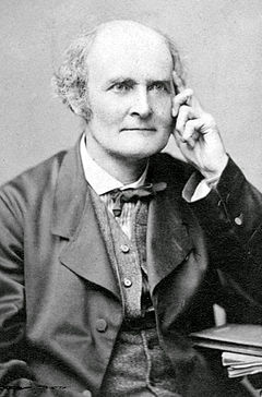
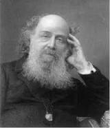
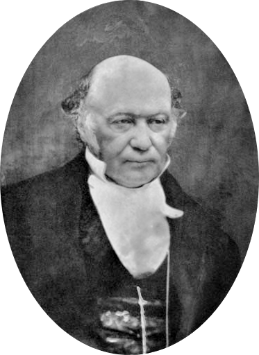
| Arthur Cayley | James Sylvester | William Hamilton |
Arthur Cayley (1821--1895) was a British mathematician, one of the founders of the modern British school of pure mathematics. As a child, Cayley enjoyed solving complex math problems for amusement. He entered Trinity College, Cambridge, where he excelled in Greek, French, German, and Italian, as well as mathematics. He worked as a lawyer for 14 years. During this period of his life, Cayley produced between two and three hundred papers. Many of his publications were results of collaboration with his friend J. J. Sylvester.
Sir William Rowan Hamilton (1805--1865) was an Irish physicist, astronomer, and mathematician, who made important contributions to classical mechanics, optics, and algebra. He was first foreign member of the American National Academy of Sciences. Hamilton had a remarkable ability to learn languages, including modern European languages, and Hebrew, Persian, Arabic, Hindustani, Sanskrit, and even Marathi and Malay. Hamilton was part of a small but well-regarded school of mathematicians associated with Trinity College in Dublin, which he entered at age 18. Paradoxically, the credit for discovering the quantity now called the Lagrangian and Lagrange's equations belongs to Hamilton. In 1835, being secretary to the meeting of the British Association which was held that year in Dublin, he was knighted by the lord-lieutenant.
James Joseph Sylvester (1814--1897) was an English mathematician. He made fundamental contributions to matrix theory, invariant theory, number theory, partition theory, and combinatorics. Sylvester was born James Joseph in London, England, but later he adopted the surname Sylvester when his older brother did so upon emigration to the United States. At the age of 14, Sylvester was a student of Augustus De Morgan at the University of London. His family withdrew him from the University after he was accused of stabbing a fellow student with a knife. Subsequently, he attended the Liverpool Royal Institution.
However, Sylvester was not issued a degree, because graduates at that time were required to state their acceptance of the Thirty-Nine Articles of the Church of England, and Sylvester could not do so because he was Jewish, the same reason given in 1843 for his being denied appointment as Professor of Mathematics at Columbia College (now University) in New York City. For the same reason, he was unable to compete for a Fellowship or obtain a Smith's prize. In 1838 Sylvester became professor of natural philosophy at University College London and in 1839 a Fellow of the Royal Society of London. In 1841, he was awarded a BA and an MA by Trinity College, Dublin. In the same year he moved to the United States to become a professor of mathematics at the University of Virginia, but left after less than four months following a violent encounter with two students he had disciplined. He moved to New York City and began friendships with the Harvard mathematician Benjamin Peirce and the Princeton physicist Joseph Henry, but in November 1843, after his rejection by Columbia, he returned to England.
One of Sylvester's lifelong passions was for poetry; he read and translated works from the original French, German, Italian, Latin and Greek, and many of his mathematical papers contain illustrative quotes from classical poetry. In 1876 Sylvester again crossed the Atlantic Ocean to become the inaugural professor of mathematics at the new Johns Hopkins University in Baltimore, Maryland. His salary was $5,000 (quite generous for the time), which he demanded be paid in gold. After negotiation, agreement was reached on a salary that was not paid in gold. In 1878 he founded the American Journal of Mathematics. In 1883, he returned to England to take up the Savilian Professor of Geometry at Oxford University. He held this chair until his death. Sylvester invented a great number of mathematical terms such as "matrix" (in 1850), "graph" (combinatorics) and "discriminant." He coined the term "totient" for Euler's totient function.
Theorem: (Cayley--Hamilton) Every square matrix A is annulled by its characteristic polynomial, that is, \( \chi ({\bf A}) = {\bf 0} , \) where \( \chi (\lambda ) = \det \left( \lambda {\bf I} - {\bf A} \right) . \) ■
Example: Consider the matrix
Theorem: For polynomials p and q and a square matrix A, \( p \left( {\bf A} \right) = q \left( {\bf A} \right) \) if and only if p and q take the same values on the spectrum (set of all eigenvalues) of A.
Theorem: The minimal polynomial ψ of a square matrix A divides any other annihilating polynomial p for which \( p \left( {\bf A} \right) = {\bf 0} . \) In particular, the minimal polynomial divides the characteristic polynomial of A. ■
From the above theorem follows that the minimal polynomial always is a product of monomials \( \lambda - \lambda_i \) for each eigenvalue λi because the characteristic polynomial contains all such multiples. So all eigenvalues must be present in the product form for a minimal polynomial.
Theorem: The minimal polynomial for a linear operator on a finite-dimensional vector space is unique.
Theorem: A square matrix A is diagonalizable if and only if its minimal polynomial is a product of simple terms: \( \psi (\lambda ) = \left( \lambda - \lambda_1 \right) \left( \lambda - \lambda_2 \right) \cdots \left( \lambda - \lambda_s \right) , \) where λ1, ... , λs are eigenvalues of matrix A. ■
Therefore, a square matrix A is not diagonalizable if and only if its minimal polynomial contains at least one multiple \( \left( \lambda - \lambda_1 \right)^m \) for m > 1.
Theorem: Every matrix that commutes with a square matrix A is a polynomial in A if and only if A is nonderogatory.
Theorem: If A is upper triangular and nonderogatory, then any solution X of the equation \( f \left( {\bf X} \right) = {\bf A} \) is upper triangular. ■
In Mathematica, one can define the minimal polynomial using the following code:
Module[{i, n = 1, qu = {},
mnm = {Flatten[IdentityMatrix[Length[a]]]}},
While[Length[qu] == 0, AppendTo[mnm, Flatten[MatrixPower[a, n]]];
qu = NullSpace[Transpose[mnm]];
n++];
First[qu].Table[x^i, {i, 0, n - 1}]]
Suppose that A is a diagonalizable \( n \times n \) matrix; this means that all its eigenvalues are not defective and there exists a basis of n linearly independent eigenvectors. Then its minimal polynomial (the polynomial of least possible degree that annihilates the matrix) is a product of simple terms:
Let \( f(\lambda ) \) be a function defined on the spectrum of the matrix A. The last condition means that every eigenvalue λi is in the domain of f, and that every eigenvalue λi with multiplicity mi > 1 is in the interior of the domain, with f being (mi — 1) times differentiable at λi. We build a function \( f\left( {\bf A} \right) \) of diagonalizable square matrix A according to James Sylvester, who was an English lawyer and music tutor before his appointment as a professor of mathematics in 1885. To define a function of a square matrix, we need to construct k Sylvester auxiliary matrices for each distinct eigenvalue \( \lambda_i , \quad i= 1,2,\ldots k: \)
This formula was formulated by James Sylvester in 1883:
J. J. Sylvester. On the equation to the secular inequalities in the planetary
theory. Philosophical Magazine, 16:267–269, 1883.
Each Sylvester's matrix \( {\bf Z}_i \) is a projection matrix on eigenspace of the corresponding eigenvalue, so \( {\bf Z}_i^2 = {\bf Z}_i , \ i = 1,2,\ldots , k; \) but \( {\bf Z}_1 {\bf Z}_2 = {\bf 0} . \)
Example: Consider a 2-by-2 matrix
Example: Consider the \( 3 \times 3 \) matrix \( {\bf A} = \begin{bmatrix} 1&4&16 \\ 18&20&4 \\ -12&-14&-7 \end{bmatrix} \) that has three distinct eigenvalues; Mathematica confirms
With Sylvester's matrices, we are able to construct arbitrary admissible functions of the given matrix. We start with the square root function \( r(\lambda ) = \sqrt{\lambda} , \) which is actually comprises of two branches \( r(\lambda ) = \sqrt{\lambda} \) and \( r(\lambda ) = -\sqrt{\lambda} . \) Indeed, choosing a particular branch, we get
We consider two other functions \( \displaystyle \Phi (\lambda ) = \frac{\sin \left( t\,\sqrt{\lambda} \right)}{\sqrt{\lambda}} \) and \( \displaystyle \Psi (\lambda ) = \cos \left( t\,\sqrt{\lambda} \right) . \) It is not a problem to determine the corresponding matrix functions
function [S1,S2,S3] = Sylvester_3X3(A)
% This function is designed to return the Sylvester Axuiliary Matrices %
% S1,S2,S3 of 3x3 diagonalizable matrix A.
% If there are less than three auxiliary matrices, it will return the proper
% amount of axuliary matrices, and return the other values as simply 0.
% Let's find the characteristic polynomial.
syms x
vec_poly = minpoly(A); % coefficients of minimal polynomial
min_poly = poly2sym(vec_poly) % create symbolic polynomial from vector of coefficients
% Eigenvalues
u = solve(min_poly,x); % distinct eigenvalues of A

E = eye(3); % 3X3 identity matrix

S1 = 0;
S2 = 0;
S3 = 0;

switch numel(u)
  case 2
    % For our first unique eigenvalue...
    S1 = (A-E*u(2))/(u(1) - u(2));
    % Now for our second...
    S2 = (A-E*u(1))/(u(2) - u(1));
  case 3
    S1 = (A - E*u(2))*(A-E*u(3))/((u(1)-u(2))*(u(1)-u(3)));
    S2 = (A - E*u(1))*(A-E*u(3))/((u(2)-u(1))*(u(2)-u(3)));
    S3 = (A - E*u(1))*(A-E*u(2))/((u(3)-u(1))*(u(3)-u(2)));
end
Example: Consider the nonderogatory (diagonalizable) \( 3 \times 3 \) matrix \( {\bf A} = \begin{bmatrix} -20&-42&-21 \\ 6&13&6 \\ 12&24&13 \end{bmatrix} \) that has only two distinct eigenvalues
Example: The matrix
\( {\bf A} = \begin{bmatrix} 1&2&3 \\ 2&3&4 \\ 2&-6&-4 \end{bmatrix} \)
has two complex conjugate eigenvalues \( \lambda = 1 \pm 2{\bf j} , \) and one real
eigenvalue \( \lambda = -2 . \) Since
\( (\lambda -1 + 2{\bf j})(\lambda -1 - 2{\bf j}) = (\lambda -1)^2 +4 , \) the Sylvester
auxiliary matrix corresponding to the real eigenvalue becomes
Sylvester's auxiliary matrices corresponding to two complex conjugate eigenvalues are also complex conjugate: % 3x3 matrix with 2 complex conjugate eigenvalues
syms lambda
A = [1 2 3; 2 3 4; 2 -6 -4] % define matrix
A_eig = eig(A) %calculate eigenvalues
resolvent = simplify(inv((lambda*eye(3)-A)))
z_2 = simplify(((A-eye(3))^2+4*eye(3))/((lambda-1)^2+4))
Z_2 = subs(z_2, lambda, -2) %plugin -2 for lambda
z1_2j = ((A+(-1+2i)*eye(3))*(A+2*eye(3)))/(4i*(3+2i))
Z1_2j = subs(z1_2j, lambda, 1+2i) %plugin 1+2j for lambda
A =
     1   2   3
     2   3   4
     2  -6  -4
A_eig =
    -2.0000 + 0.0000i
     1.0000 + 2.0000i
     1.0000 - 2.0000i
where \( \sigma_1 = \lambda^3 + \lambda +10 \)
z2 =
\(
\begin{pmatrix}
\frac{14}{\sigma_1} & -\frac{14}{\sigma_1} & -\frac{7}{\sigma_1} \\
\frac{12}{\sigma_1} & -\frac{12}{\sigma_1} & -\frac{6}{\sigma_1} \\
-\frac{22}{\sigma_1} & \frac{22}{\sigma_1} & \frac{11}{\sigma_1}
\end{pmatrix} \)
where \( \sigma_1 = (\lambda -1)^2 +4 \)
z_2 =
\(
\begin{pmatrix}
\frac{14}{13}&1-\frac{14}{13}&-\frac{7}{13} \\ \frac{12}{13}&-\frac{12}{13}
&-\frac{6}{13} \\ -\frac{22}{13}&\frac{22}{13}&\frac{11}{13}
\end{pmatrix} \)
z1_2j =
A =
    -0.0385 - 0.8077i   0.5385 + 0.
    -0.4615 - 1.1923i   0.9615 + 0.
     0.8462 + 0.7692i  -0.8462 + 0.
Z1_2j =
\(
\begin{pmatrix}
- \frac{1}{26} - \frac{21}{26}\,i & \frac{7}{13} + \frac{4}{13}\, i & \frac{7}{26} \\
- \frac{6}{13} - \frac{31}{26}\,i & \frac{25}{26} + \frac{5}{26}\, i & \frac{3}{13} \\
\frac{11}{13} + \frac{10}{13}\,i & - \frac{11}{13} + \frac{3}{13}\, i & \frac{1}{13} +
\end{pmatrix} \)
This auxiliary matrix is a projection; as so \( {\bf Z}_{-2} {\bf Z}_{-2} = {\bf Z}_{-2}^2 = {\bf Z}_{-2}^3 = {\bf Z}_{-2} . \)