Consider a homogeneous systems of linear differential equations with constant coefficients:
\[
\begin{split}
\dot{y}_1 &= a_{11} y_1 + a_{12} y_2 + \cdots + a_{1n} y_n , \\
\dot{y}_2 &= a_{21} y_1 + a_{22} y_2 + \cdots + a_{2n} y_n , \\
\vdots & \qquad \vdots \\
\dot{y}_n &= a_{n1} y_1 + a_{n2} y_2 + \cdots + a_{nn} y_n , \\
\end{split}
\]
which we rewrite in compact vector form
\[
\dot{\bf y} (t) = {\bf A} \,{\bf y} (t) \qquad \mbox{or} \qquad \frac{{\text
d}{\bf y}}{{\text d} t} = {\bf A} \,{\bf y} (t),
\]
where A is the constant n-by-n matrix of coefficients
and y is the n-dimensional column vector of unknown
functions:
\[
{\bf A} = \begin{bmatrix} a_{11} & a_{12} & \cdots & a_{1n} \\
a_{21} & a_{22} & \cdots & a_{2n} \\
\vdots & \vdots & \ddots & \vdots \\
a_{n1} & a_{n2} & \cdots & a_{nn}
\end{bmatrix} , \qquad {\bf y} (t) = \begin{bmatrix} y_1 \\ y_2 \\
\vdots \\ y_n \end{bmatrix} .
\]
Its general solution is known to be
\[
{\bf y} (t) = e^{{\bf A}\,t} \, {\bf c} ,
\]
where c is n column vector of arbitrary constants. The
matrix function \( {\bf \Phi} (t) = e^{{\bf A}\,t}
\) is called the fundamental matrix or propagator for
the above vector differential equation \( \dot{\bf
y} = {\bf A}\,{\bf y}. \) Since the exponential matrix
function \( {\bf \Phi} (t) \) is the
unique solutions to the following matrix differential
equation
\[
\frac{{\text d} }{{\text d} t}\,{\bf \Phi} = {\bf A} \,{\bf \Phi} (t),
\qquad {\bf \Phi} (0) = {\bf I} ,
\]
where I is the identity n-by-n matrix, the vector
function y(t) satisfies the initial condition
\( {\bf y} (0) = e^{{\bf A}\,0} \, {\bf c} = {\bf c} . \)
\( \dot{\bf x} = {\bf A}\,{\bf x}. \)
Example: engineering applications.
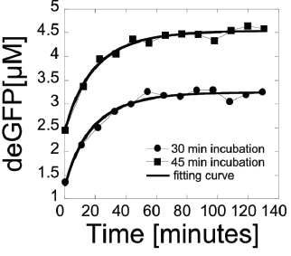
In this example, we examine endogenous mRNA inactivation to better understand gene expression dynamics. The protein used is deGFP, which is a highly translatable green flourescent protein. The following differential equations describe the rate of change over time of the concentration of deGFP mRNA (m), dark deGFP (deGFPd), and flourescent deGFP (deGFPf).
\begin{align*}
\frac{\text d}{{\text d} t}\, m(t) &= -B\,m(t) ,
\\
\frac{\text d}{{\text d} t}\,\mbox{deGRPd}(t) &= a\,m(t) -k\,\mbox{deGFPd} (t),
\\
\frac{\text d}{{\text d} t} \,\mbox{deGFPf} (t)&= k\,\mbox{deGFPd}(t) .
\end{align*}
clear;
syms B m(t) deGFPd(t) a k deGFPf(t);
eqns=[diff(m)==-B*m;diff(deGFPd)==a*m-k*deGFPd;diff(deGFPf)==k*deGFPd]
\[
m(0) = \frac{1}{4}, \qquad \mbox{deGFPd} (0) = \frac{1}{4} , \qquad
\mbox{deGFPf}(0) =0 .
\]
cond=[deGFPf(0)==0;deGFPd(0)==0.25;m(0)==0.25]We solve the above differential equations using these initial conditions to find equations for the concentration of each item in terms of time.
soln=dsolve([eqns;cond]);
deGFPd_(t)=soln.deGFPd
\[
\mbox{deGFPd} (t) = e^{-kt}\,\frac{B+a-k}{4\left( B-k \right)} -
\frac{a}{4\left( B-k \right)} \, e^{-Bt} .
\]
m_(t)=soln.m
\[
m(t) = \frac{1}{4}\, e^{-Bt} .
\]
deGFPf_(t)=soln.deGFPf
\[
\mbox{deGFPf}(t) = \frac{B+a}{4\,B} - \frac{B+a-k}{4\left( B-k \right)}\, e^{-kt} + \frac{ak}{4B\left( B-k \right)}\, e^{-Bt} .
\]
The study gives the final solved equation as
\[
\mbox{deGFP}_f (t) = \frac{a\,m_0}{B\left( B-k \right)} \left( k\,e^{-Bt} - k +B - B\, e^{-kt} \right) .
\]
where m0 is the concentration of active mRNA when
transcription is ended. This equation is algebraically equivalent to the
result given by matlab (once
some higher order terms are removed). This model follows the collected data
closely as shown on page 5 of Shin and Noireaux (2010).
Complete