MATLAB Tutorial for the Second Course, Part 2.3: Forced Duffing equation

We consider the Duffing oscillator under periodic driven force:

\begin{equation} \label{EqFD.1} \ddot{x} + x + \varepsilon \,x^3 = F\,\cos \omega t, \end{equation}

and

\begin{equation} \label{EqFD.2} \ddot{x} + x + \varepsilon \,x^3 = F\,\sin \omega t. \end{equation}

Here ε is a small parameter and F is the amplitude of oscillating force. We consider both equations, \eqref{EqFD.1} and \eqref{EqFD.2} under homogeneous conditions

\[ x(0) = 0 , \qquad \dot{x}(0) = 0. \]

Using the spring analogy for this differential equation, for a fixed value of ω and small value of amplitude F, the spring oscillates quite nicely; as F is increased the oscillations increase in amplitude until the threshold is reached and the spring breaks (the solution becomes unbounded).

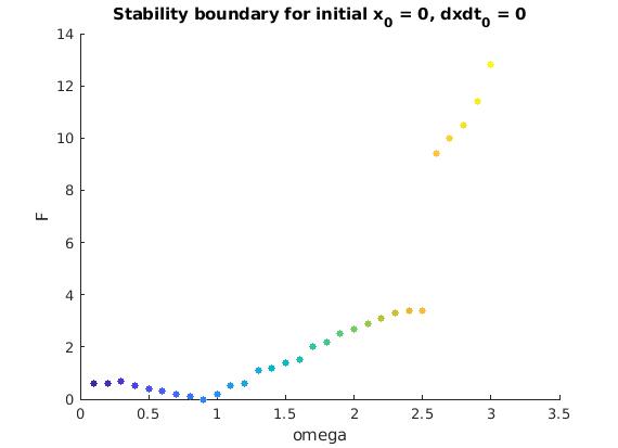
For the initial value problem

\[ \ddot{x} + x - \frac{1}{6} \,x^3 = F\,\cos \omega t, \qquad x(0) = 0, \quad \dot{x}(0) =0 , \]

we try to determine the boundary on (F, ω)-plane where solutions of the Duffing equation above are bounded.


clear all
clc 

epsilon = -1/6;
tmax = 150;
oms = 30;

warning('off','all')
opts = odeset('Reltol',1e-13,'AbsTol',1e-14);
t_span = [0, tmax];

init   = [0, 0];
omega = 0.1;
tmaxi = tmax;

stability = zeros(oms,2);
for i = 1:oms
    F = 0;
    tmax = tmaxi;
    disp(omega)
    while tmax > tmaxi - 2
        F = F + 0.5;    
        [t, x] = ode113(@(t,w) duff(t,w,epsilon,F,omega), t_span, init, opts);
        tmax = max(t);       
    end
    
    while tmax < tmaxi - 2
        F = F - 0.1;     
        [t, x] = ode113(@(t,w) duff(t,w,epsilon,F,omega), t_span, init, opts);
        tmax = max(t);        
    end
   
    stability(i,:) = [omega, F];
    omega = omega + 0.1;
end

figure
sz = 25;
c = linspace(1,10,oms);
scatter(stability(:,1),stability(:,2),sz,c,'filled')
ylabel('F')
xlabel('omega')
title('Stability boundary for initial x_0 = 0, dxdt_0 = 0')
init   = [0, 1];
omega = 0.1;

stability = zeros(oms,2);
for i = 1:oms
    F = 0;
    tmax = tmaxi;
    disp(omega)
    while tmax > tmaxi - 2
        F = F + 0.5;    
        [t, x] = ode113(@(t,w) duff(t,w,epsilon,F,omega), t_span, init, opts);
        tmax = max(t);       
    end
    
    while tmax < tmaxi - 2        
        F = F - 0.1;
        [t, x] = ode113(@(t,w) duff(t,w,epsilon,F,omega), t_span, init, opts);
        tmax = max(t);        
    end
    
    stability(i,:) = [omega, F];
    omega = omega + 0.1;
end

figure
scatter(stability(:,1),stability(:,2),sz,c,'filled')
ylabel('F')
xlabel('omega')
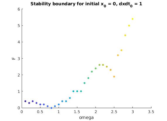
title('Stability boundary for initial x_0 = 0, dxdt_0 = 1')

function dwdt = duff(t,w,epsilon,F,omega)
x = w(1);
y = w(2);
dxdt = y;
dydt = - x - epsilon * x^3 + F * cos(omega*t);
dwdt = [dxdt;dydt];
end

The boundary of the domain where solutions of the Duffing equations subject to the homogeneous initial conditions are bounded. The boundary of the domain where solutions of the Duffing equations subject to the initial conditions x(0) = 0, x'(0) = 1, are bounded. matlab code.

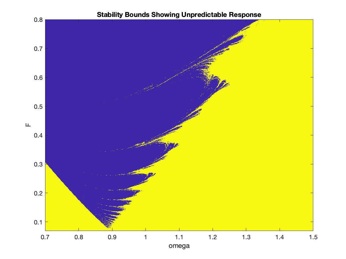
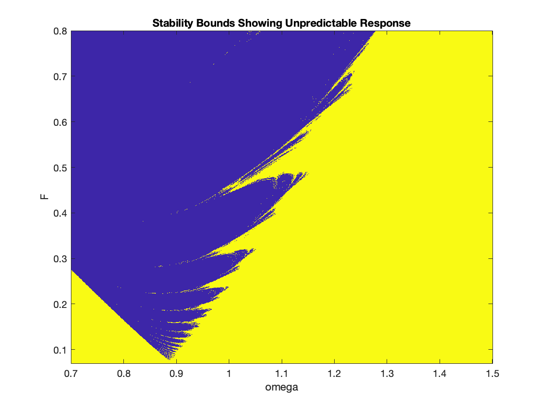
There are at least two significant features observable on this stability boundary curve. The first is the rather sharp dip in the curve forming a local and global minimum. For this initial value problem, the global and local minimum occurs for ω ≈ 0.8852, discovered by Davis.

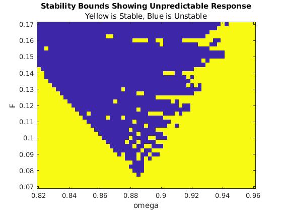
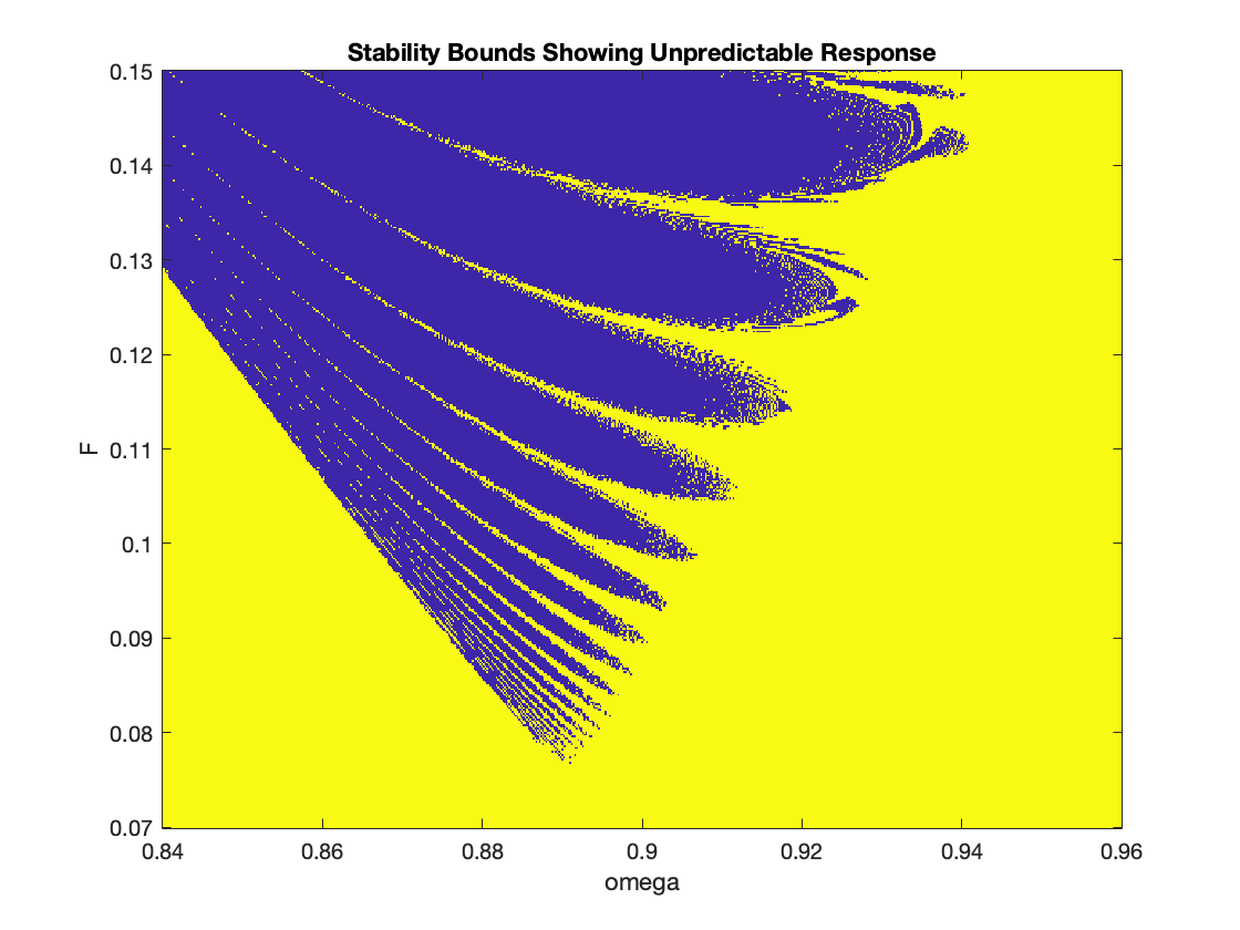
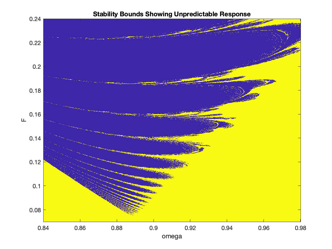
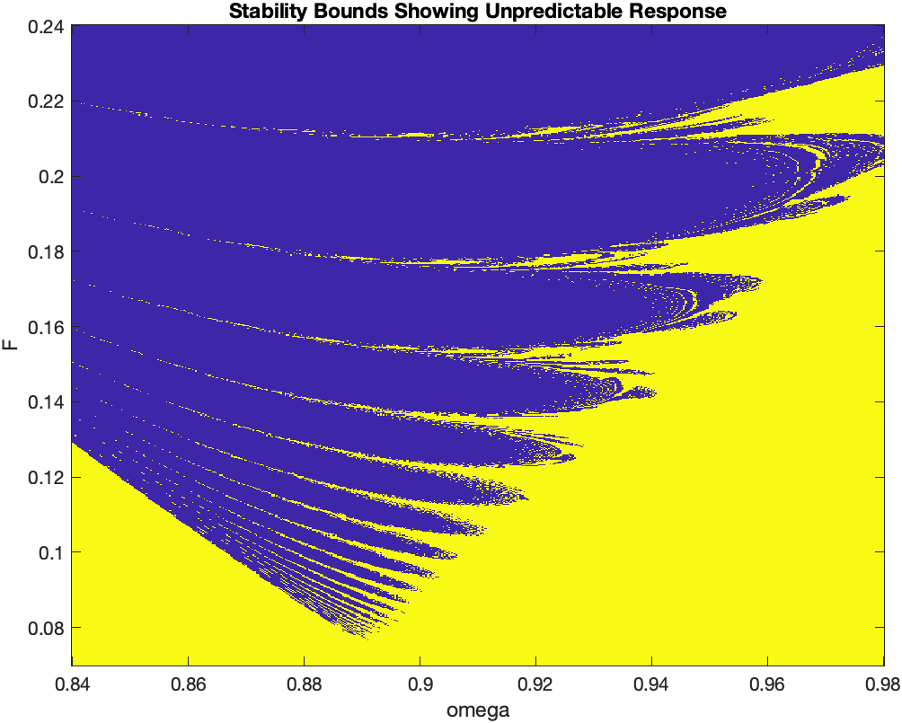
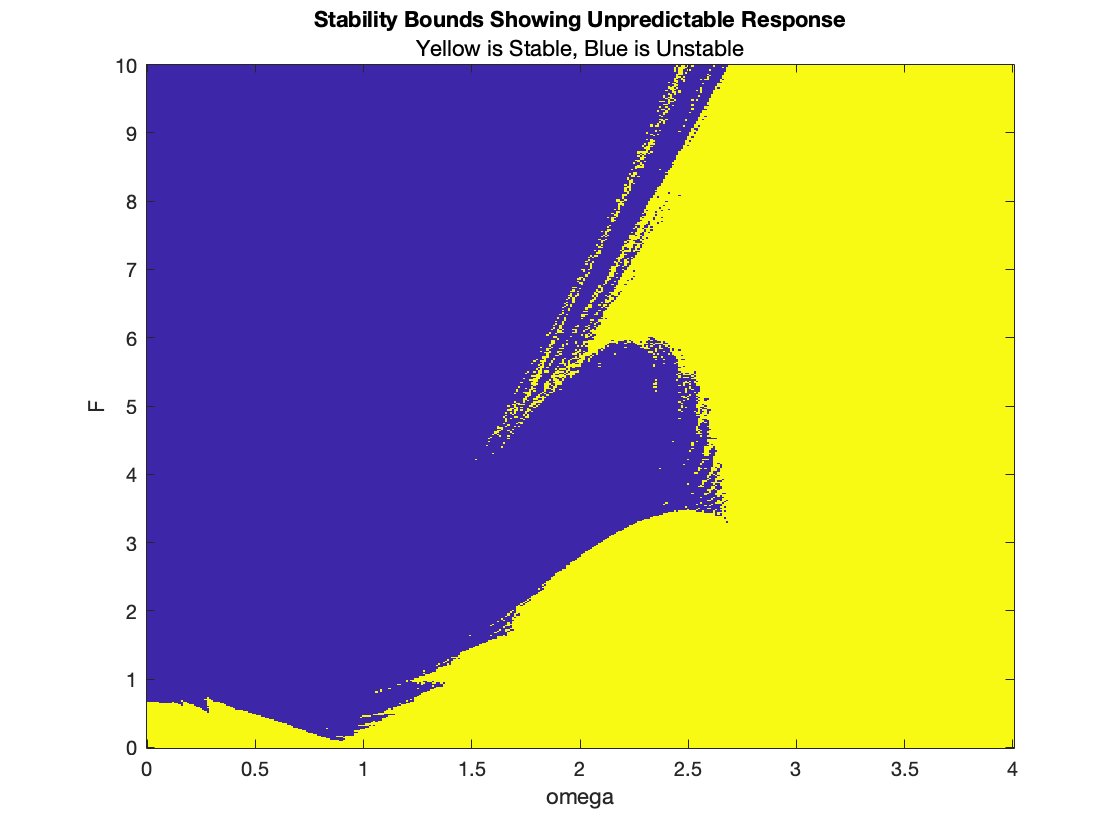
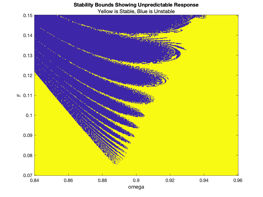
To make the boundary more clear, we write the code that produces an output with two colors---blue where values of (F, ω) cause unbounded solutions, and yellow when these values lead to bounded solutions.


clear all
clc 

% runtime is about 10 sec for low precision
% prints out the omega values it solving for so you can check if the code
% is stuck somewhere
tic;
epsilon = -1/6;
tmax = 150;

% low precision -- misses a lot of detail, for quick testing
% runtime: 10 sec
oms = 0.820:0.0025:0.960;
fs = 0.070:0.0025:0.170;

warning('off','all')
opts = odeset('Reltol',1e-13,'AbsTol',1e-14);
t_span = [0, tmax];

init   = [0, 0];

stability = zeros(length(fs),length(oms));
frow = 1:length(fs);
for i = 1:length(oms)
    disp(oms(i))
    temp = zeros(length(fs),1);
    
    for f = frow
        F = fs(f);
        omega = oms(i);
        warning('off','all')
        [t, x] = ode113(@(t,w) duff(t,w,epsilon,F,omega), t_span, init, opts); 
        if max(t) > tmax-2
            temp(f) = 1;
        end
    end    
    stability(:,i) = temp;
end

figure
s = imagesc([oms(1) oms(length(oms))],[fs(1) fs(length(fs))],stability);
ax = gca;
ax.YDir = 'normal';
title("Stability Bounds Showing Unpredictable Response")
subtitle("Yellow is Stable, Blue is Unstable")
xlabel("omega")
ylabel("F")
hold off

toc;

function dwdt = duff(t,w,epsilon,F,omega)
x = w(1);
y = w(2);
dxdt = y;
dydt = - x - epsilon * x^3 + F * cos(omega*t);
dwdt = [dxdt;dydt];
end

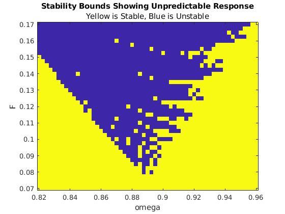
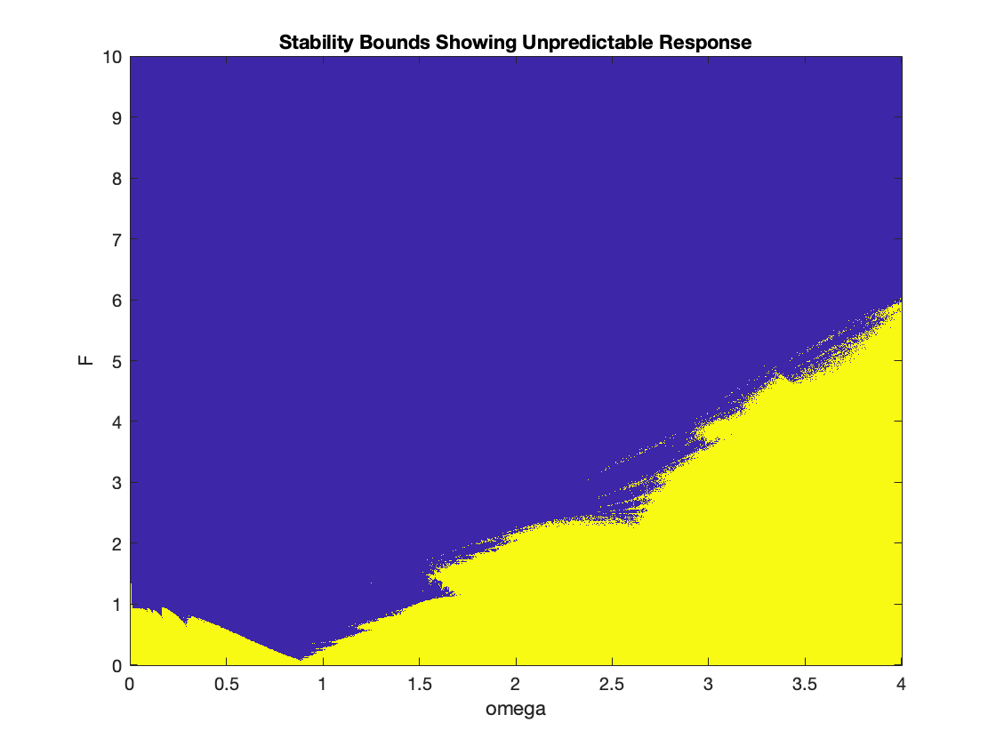
We repeat the same calculation when the forcing functions is sine, as in Eq.\eqref{EqFD.2}


clear all
clc 
% runtime is about 10 sec for low precision
% prints out the omega values it solving for so you can check if the code
% is stuck somewhere

tic;

epsilon = -1/6;
tmax = 150;

% low precision -- misses a lot of detail, for quick testing
% runtime: 10 sec
oms = 0.820:0.0025:0.960;
fs = 0.070:0.0025:0.170;

warning('off','all')
opts = odeset('Reltol',1e-13,'AbsTol',1e-14);
t_span = [0, tmax];
init   = [0, 0];

stability = zeros(length(fs),length(oms));
frow = 1:length(fs);

for i = 1:length(oms)
    disp(oms(i))
    temp = zeros(length(fs),1);
    
    for f = frow
        F = fs(f);
        omega = oms(i);
        warning('off','all')
        [t, x] = ode113(@(t,w) duff(t,w,epsilon,F,omega), t_span, init, opts); 
        if max(t) > tmax-2
            temp(f) = 1;
        end
    end
    stability(:,i) = temp;    
end

figure
s = imagesc([oms(1) oms(length(oms))],[fs(1) fs(length(fs))],stability);
ax = gca;
ax.YDir = 'normal';
title("Stability Bounds Showing Unpredictable Response")
subtitle("Yellow is Stable, Blue is Unstable")
xlabel("omega")
ylabel("F")
hold off

toc;

function dwdt = duff(t,w,epsilon,F,omega)
x = w(1);
y = w(2);
dxdt = y;
dydt = - x - epsilon * x^3 + F * sin(omega*t);
dwdt = [dxdt;dydt];
end

The resulting stability boundary obtained initially resembles the one obtained by Davis as things go along quite nicely until ω reaches 2.6 where a sudden and unexpected jump in the boundary occurs. Clearly this appears to be similar to a jump discontinuity in the stability boundary curve.

This jump occurs between ω = 2.66 and F = 3.360 and ω = 2.67 and F = 9.901. For values of ω larger than 2.67, the corresponding F values on the boundary curve grow large; for example for ω = 3.1, the corresponding boundary F-value is 14.893. For reasons of scale, we did not calculate boundary values for ω larger than 3.1. We call the value ω = 2.67 the jump frequency although the term high resonance frequency might be appropriate. In the spring analogy, this means that for ω just less than the jump frequency it takes only a moderate amplitude (force) to brake the spring, but for ω larger than the jump frequency it takes significantly more amplitude to reach the breaking point.

First, we try to determine the boundary on (F, ω)-plane where solutions of the Duffing equation \eqref{EqFD.2} are bounded.


clear all
clc

Next, we repeat our calculations for boundary determination with sine function, Eq.\eqref{EqFD.2}


clear all
clc

As you see, these codes provide only rough estimation of the boundary. Therefore, we improve the code and run it on supercomputer.


clear all
clc

epsilon = -1/6;
tmax = 150;
oms = 30;

warning('off','all')
opts = odeset('Reltol',1e-13,'AbsTol',1e-14);
t_span = [0, tmax];

init   = [0, 0];
omega = 0.1;
tmaxi = tmax;

stability = zeros(oms,2);

for i = 1:oms 
    F = 0;
    tmax = tmaxi;
    disp(omega)
    
    while tmax > tmaxi - 2
        F = F + 0.5;
        [t, x] = ode113(@(t,w) duff(t,w,epsilon,F,omega), t_span, init, opts);
        tmax = max(t);       
    end
    
    while tmax < tmaxi - 2
        F = F - 0.1;
        [t, x] = ode113(@(t,w) duff(t,w,epsilon,F,omega), t_span, init, opts);
        tmax = max(t);        
    end
    
    stability(i,:) = [omega, F];
    omega = omega + 0.1;
end

figure
sz = 25;
c = linspace(1,10,oms);
scatter(stability(:,1),stability(:,2),sz,c,'filled')
ylabel('F')
xlabel('omega')
title('Stability boundary for initial x_0 = 0, dxdt_0 = 0')

init   = [0, 1];
omega = 0.1;

stability = zeros(oms,2);

for i = 1:oms
    F = 0;
    tmax = tmaxi;
    disp(omega)
    
    while tmax > tmaxi - 2
        F = F + 0.5;
        [t, x] = ode113(@(t,w) duff(t,w,epsilon,F,omega), t_span, init, opts);
        tmax = max(t);       
    end
    
    while tmax < tmaxi - 2
        F = F - 0.1;
        [t, x] = ode113(@(t,w) duff(t,w,epsilon,F,omega), t_span, init, opts);
        tmax = max(t);        
    end
    
    stability(i,:) = [omega, F];
    omega = omega + 0.1;
    end

figure
scatter(stability(:,1),stability(:,2),sz,c,'filled')
ylabel('F')
xlabel('omega')
title('Stability boundary for initial x_0 = 0, dxdt_0 = 1')

function dwdt = duff(t,w,epsilon,F,omega)
x = w(1);
y = w(2);
dxdt = y;
dydt = - x - epsilon * x^3 + F * cos(omega*t);
dwdt = [dxdt;dydt];
end


Forcing function: cos(ωt), 0.84 < ω < 0.98		Forcing function: sin(ωt), 0.84 < ω < 0.98


Forcing function: cos(ωt), 0 < ω < 4		Forcing function: sin(ωt), 0 < ω < 4


Forcing function: cos(ωt), 0.7 < ω < 1.5		Forcing function: cos(ωt), 0.84 < ω < 0.98 & 0.07 < F < 0.15

Davis, H.T., Introduction to Nonlinear Differential and Integral Equations, 1962, (New York: Dover Publications).
Duffing, G., 1918, Erzwungene Schwingungen bei veränderlicher Eigenfrequenz, PhD Thesis, Braunschweig: Sammlung Vieweg.
Fay, T.H., Nonlinear resonance and Duffing's spring equation, International Journal of Mathematical Education in Science and Technology, 2006, Vol. 37, No. 5, pp. 593--599. https://doi.org/10.1080/00207390600594887
Fay
617.